Multivariable Control Systems
Multivariable Control Systems. Ali Karimpour Assistant Professor Ferdowsi University of Mashhad. Chapter 2. Introduction to Multivariable Control. Topics to be covered include:. Multivariable Connections Multivariable Poles Multivariable Zeros Directions of Poles and Zeros


Multivariable Control Systems
E N D
Presentation Transcript
Multivariable Control Systems Ali Karimpour Assistant Professor Ferdowsi University of Mashhad
Chapter 2 Introduction to Multivariable Control Topics to be covered include: • Multivariable Connections • Multivariable Poles • Multivariable Zeros • Directions of Poles and Zeros • Smith Form of a Polynomial Matrix • Smith-McMillan Forms • Matrix Fraction Description (MFD) • Scaling • Performance Specification • Trade-offs in Frequency Domain • Bandwidth and Crossover Frequency
Generally Multivariable Connections • Cascade (series) interconnection of transfer matrices • Parallel interconnection of transfer matrices
Multivariable Connections • Feedback interconnection of transfer matrices A useful relation in multivariable is push-through rule Exercise 1: Proof the push-through rule
MIMO rule: To derive the output of a system, start from the output and write down the blocks as you meet them when moving backward (against the signal flow) towards the input. If you exit from a feedback loop then include a term or according to the feedback sign where L is the transfer function around that loop (evaluated against the signal flow starting at the point of exit from the loop). Parallel branches should be treated independently and their contributions added together. Multivariable Connections
Multivariable Connections Example 2-1: Derive the transfer function of the system shown in figure
Definition 2-1: The poles of a system with state-space description are eigenvalues of the matrix A. The pole polynomial or characteristic polynomial is defined as Multivariable Poles ( State Space Description ) Thus the system’s poles are the roots of the characteristic polynomial Note that if A does not correspond to a minimal realization then the poles by this definition will include the poles (eigenvalues) corresponding to uncontrollable and/or unobservable states.
Theorem 2-1 The pole polynomial corresponding to a minimal realization of a system with transfer function G(s) is the least common denominator of all non-identically-zero minors of all orders of G(s). A minor of a matrix is the determinant of the square matrix obtained by deleting certain rows and/or columns of the matrix. Multivariable Poles ( Transfer Function Description )
Example 2-4 The non-identically-zero minors of order 1 are The non-identically-zero minor of order 2 are By considering all minors we find their least common denominator Multivariable Poles ( Transfer Function Description )
Exercise 2: Consider the state space realization Multivariable Poles a- Find the poles of the system directly through state space form. b- Find the transfer function of system ( note that the numerator and the denominator of each element must be prime ). c- Find the poles of the system through its transfer function.
Laplace transform Let Multivariable Zeros ( State Space Description ) The zeros are then the values of s=z for which the polynomial system matrix P(s) loses rank resulting in zero output for some nonzero input. Then the zeros are found as non trivial solutions of This is solved as a generalized eigenvalue problem.
Multivariable Zeros ( State Space Description ) For square systems with m=p inputs and outputs and n states, limits on the number of transmission zeros are:
Example 2-5: Consider the state space realization Multivariable Zeros ( State Space Description )
is a zero of G(s) if the rank of is less than the normal rank of G(s). The zero polynomial is defined as . Where is the number of finite zeros of G(s). Multivariable Zeros ( Transfer Function Description ) Definition 2-2
The zero polynomialz(s) corresponding to a minimal realization of the system is the greatest common divisor of all the numerators of all order-r minors of G(s) where r is the normal rank of provided that these minors have been adjusted in such a way as to have the pole polynomial as their denominators. Multivariable Zeros ( Transfer Function Description ) Theorem 2-2
according to example 2-4 the pole polynomial is: The minors of order 2 with as their denominators are Multivariable Zeros ( Transfer Function Description ) Example 2-9 The greatest common divisor of all the numerators of all order-2 minors is
Exercise 3: Consider the state space realization Multivariable Poles a- Find the zeros of the system directly through state space form. b- Find the transfer function of system ( note that the numerator and the denominator of each element must be prime ). c- Find the zeros of the system through its transfer function.
Let G(s) have a zero at s = z, Then G(s) losses rank at s = z and there will exist nonzero vectors and such that is input zero direction and is output zero direction Directions of Poles and Zeros Zero directions: We usually normalize the direction vectors to have unit length
is input pole direction and is output pole direction Directions of Poles and Zeros Pole directions: Let G(s) have a pole at s = p. Then G(p) is infinite and we may somewhat crudely write
Example: Input zero direction Output zero direction Directions of Poles and Zeros It has a zero at z = 4 and a pole at p = -2 .
Example: Input pole direction Output pole direction Directions of Poles and Zeros It has a zero at z = 4 and a pole at p = -2 . ??!!
Suppose that is a polynomial matrix. Smith formof is denoted by , and it is a pseudo diagonal in thefollowing form is a factor of and Smith Form of a Polynomial Matrix
gcd {all monic minors of degree 1} gcd {all monic minors of degree 2} gcd {all monic minors of degree r} is a factor of and Smith Form of a Polynomial Matrix ……………………………………………………….. ………………………………………………………..
Smith Form of a Polynomial Matrix The three elementary operations for a polynomial matrix are used to find Smith form. • Multiplying a row or column by a constant; • Interchanging two rows or two columns; and • Adding a polynomial multiple of a row or column to another • row or column.
Example 2-11 Exercise 4: Derive R(s) and L(s) that convert to Smith Form of a Polynomial Matrix
Let be an m × p matrix transfer function, where arerationalscalar transfer functions, G(s) can be represented by: Then, is Smith McMillan form of G(s) and can be derived directly by Smith-McMillan Forms Theorem 2-3 (Smith-McMillan form) Where Π(s) is an m× p polynomial matrix of rank r and DG(s) is the least common multiple of the denominators of all elements of G(s) .
Smith-McMillan Forms Theorem 2-3 (Smith-McMillan form)
Smith-McMillan Forms Example 2-13
polynomial polynomial polynomial polynomial Matrix Fraction Description (MFD) This is a Right Matrix Fraction Description (RMFD) This is a Left Matrix Fraction Description (LMFD)
Let is a matrix and its the Smith McMillan is Let define: Matrix Fraction Description (MFD) A model structure that is related to the Smith-McMillan form is matrix fraction description (MFD). • Right matrix fraction description (RMFD) • Left matrix fraction description (LMFD)
Matrix Fraction Description (MFD) We know that This is known as a right matrix fraction description (RMFD) where
Matrix Fraction Description (MFD) We know that This is known as a left matrix fraction description (LMFD) where
We can show that the MFD is not unique, because, for any nonsingular matrix we can write G(s) as: Where is said to be a right common factor. When the only right common factors of and is unimodular matrix, then, we Say that the RMFD is irreducible. Matrix Fraction Description (MFD) It is easy to see that when a RMFD is irreducible, then
Matrix Fraction Description (MFD) Example 2-16 RMFD:
Matrix Fraction Description (MFD) Example 2-16 LMFD:
Performance Specification • Nominal stability NS: The system is stable with no model uncertainty. • Nominal Performance NP: The system satisfies the performance • specifications with no model uncertainty. • Robust stability RS: The system is stable for all perturbed plants • about the nominal model up to the worst case model uncertainty. • Robust performance RP: The system satisfies the performance • specifications for all perturbed plants about the nominal model up • to the worst case model uncertainty.
Performance Specification • Time Domain Performance • Frequency Domain Performance
Time Domain Performance Although closed loop stability is an important issue, the realobjective of control is to improve performance, that is, to make the output y(t) behave in a more desirable manner. Actually, the possibility of inducing instability is one of the disadvantages of feedback control which has to be traded off against performance improvement. The objective of this section is to discuss ways of evaluating closed loop performance.
Step response of a system Time Domain Performance • Rise time, tr , the time it takes for the output to first reach 90% of its final value, which is usually required to be small. • Settling time, ts , the time after which the output remains within 5% ( or 2%) of its final value, which is usually required to be small. • Overshoot, P.O, the peak value divided by the final value, which should typically be less than 20% or less.
Step response of a system Time Domain Performance • Decay ratio, the ratio of the second and first peaks, which should typically be 0.3 or less. • Steady state offset,ess, the difference between the final value and the desired final value, which is usually required to be small.
Step response of a system Time Domain Performance • Excess variation, the total variation (TV) divided by the overall change at steady state, which should be as close to 1 as possible. The total variation is the total movement of the output as shown.
ISE: Integral squared error • IAE : Integral absolute error • ITSE: Integral time weighted squared error • ITAE: Integral time weighted absolute error Time Domain Performance
Bode plot of Frequency Domain Performance Let L(s) denote the loop transfer function of a system which is closed-loop stable under negative feedback.
Nyquist plot of Frequency Domain Performance Let L(s) denote the loop transfer function of a system which is closed-loop stable under negative feedback.
More generally, to maintain closed-loop stability, the Nyquist stability condition tells us that the number of encirclements of the critical point -1 by must not change. Frequency Domain Performance Stability margins are measures of how close a stable closed-loop system is to instability. From the above arguments we see that the GM and PM provide stability margins for gain and delay uncertainty. Thus the actual closest distance to -1 is a measure of stability
Complementary sensitivity function Sensitivity function Frequency Domain Performance One degree-of-freedom configuration The maximum peaks of the sensitivity and complementary sensitivity functions are defined as
Frequency Domain Performance Thus one may also view Ms as a robustness measure.
Frequency Domain Performance There is a close relationship between MS and MT and the GM and PM. For example, with MS = 2 we are guaranteed GM > 2 and PM >29˚. For example, with MT = 2 we are guaranteed GM > 1.5 and PM >29˚.
Complementary sensitivity function Sensitivity function Trade-offs in Frequency Domain One degree-of-freedom configuration