Multivariable Control Systems
Multivariable Control Systems. Ali Karimpour Assistant Professor Ferdowsi University of Mashhad. Chapter 3. Limitation on Performance in MIMO Systems. Topics to be covered include:. Scaling and Performance. Shaping Closed-loop Transfer Functions. Fundamental Limitation on Sensitivity.


Multivariable Control Systems
E N D
Presentation Transcript
Multivariable Control Systems Ali Karimpour Assistant Professor Ferdowsi University of Mashhad
Chapter 3 Limitation on Performance in MIMO Systems Topics to be covered include: • Scaling and Performance • Shaping Closed-loop Transfer Functions • Fundamental Limitation on Sensitivity • Fundamental Limitation: Bounds on Peaks • Functional Controllability • Limitations Imposed by Time Delays • Limitations Imposed by RHP Zeros • Limitations Imposed by Unstable (RHP) Poles
Introduction One degree-of-freedom configuration • Performance, good disturbance rejection • Performance, good command following • Mitigation of measurement noise on output
Scaling and Performance • For any reference r(t) between -R and R and any disturbance d(t) between -1 and 1, keep the output y(t) within the range r(t)-1 to r(t)+1 (at least most of the time), using an inputu(t) within the range -1 to 1. • For any disturbance |d(ω)| ≤ 1 and any reference |r(ω)|≤ R(ω), the performance requirement is to keep at each frequency ω the control error |e(ω)|≤1 using an input |u(ω)|≤1.
Shaping Closed-loop Transfer Functions Many design procedure act on the shaping of the open-loop transfer functionL. An alternative design strategy is to directly shape the magnitudes of closed-loop transfer functions, such as S(s) and T(s). Such a design strategy can be formulated as an H∞ optimal control problem, thus automating the actual controller design and leaving the engineer with the task of selecting reasonable bounds “weights” on the desired closed-loop transfer functions.
The termsH∞ and H2 The H∞ norm of a stable transfer function matrix F(s) is simply define as, We are simply talking about a design method which aims to press down the peak(s) of one or more selected transfer functions. Now, the term H∞ which is purely mathematical, has now established itself in the control community. In literature the symbol H∞stands for the transfer function matrices with bounded H∞-norm which is the set of stable and proper transfer function matrices.
The termsH∞ and H2 The H2 norm of a stable transfer function matrix F(s) is simply define as, Similarly, the symbol H2 stands for the transfer function matrices with bounded H2-norm, which is the set of stable and strictly proper transfer function matrices. Note that the H2norm of a semi-proper transfer function is infinite, whereas its H∞ norm is finite. Why?
Weighted Sensitivity As already discussed, the sensitivity function Sis a very good indicator of closed-loop performance (both for SISO and MIMO systems). Why Sis a very good indicator of closed-loop performance in many literatures? The mainadvantage of considering S is that because we ideally want S to be small, it is sufficient to consider just its magnitude, ||S|| that is, we need not worryabout its phase.
Weighted Sensitivity Typical specifications in terms of S include: • Minimum bandwidth frequency ωB*. • Maximum tracking error at selected frequencies. • System type, or alternatively the maximum steady-state tracking error, A. • Shape of S over selected frequency ranges. • Maximum peak magnitude of S, ||S(jω)||∞≤M The peak specification prevents amplification of noise at high frequencies, and also introduces a margin of robustness; typically we select M=2
Weighted Sensitivity Mathematically, these specifications may be captured simply by an upper bound The subscript P stands for performance
plot of Weighted Selection
For example, for disturbance rejection Weighted Selection A weight which asks for a slope -2 for L at lower frequencies is The insight gained from the previous section on loop-shaping design is very useful for selecting weights. It then follows that a good initial choice for the performance weight is to let wP(s) look like |Gd(jω)| at frequencies where|Gd(jω)| >1
Stacked Requirements: Mixed Sensitivity The specification ||wPS||∞<1 puts a lower bound on the bandwidth, but not an upper one, and nor does it allow us to specify the roll-off of L(s) above the bandwidth. To do this one can make demands on another closed-loop transfer function For SISO systems, N is a vector and
For example, In general, with n stacked requirements the resulting error is at most Stacked Requirements: Mixed Sensitivity The stacking procedure is selected for mathematical convenience as it does not allow us to exactly specify the bounds. We want to achieve This is similar to, but not quite the same as the stacked requirement
Let denote the optimal H∞norm. The practical implication is that, except for at most a factor the transfer functions will be close to times the bounds selected by the designer. This gives the designer a mechanism for directly shaping the magnitudes of Solving H∞ Optimal Control Problem After selecting the form of N and the weights, the H∞optimal controller is obtained by solving the problem
Solving H∞ Optimal Control Problem Example 3-1 The control objectives are: • Command tracking: The rise time (to reach 90% of the final value) • should be less than 0.3 second and the overshoot should be less than 5%. 2. Disturbance rejection: The output in response to a unit step disturbance should remain within the range [-1,1] at all times, and it should return to 0 as quickly as possible (|y(t)| should at least be less than 0.1 after 3 seconds). 3. Input constraints: u(t) should remain within the range [-1,1] at all times to avoid input saturation (this is easily satisfied for most designs).
Solving H∞ Optimal Control Problem Consider an H∞ mixed sensitivity S/KS design in which It was stated earlier that appropriate scaling has been performed so that the inputs should be about 1 or less in magnitude, and we therefore
Solving H∞ Optimal Control Problem We need control till 10 rad/sec to reduce disturbance and a suitable rise time. Overshoot should be less than 5% so let MS<1.5
Solving H∞ Optimal Control Problem For this problem, we achieved an optimal H∞ norm of 1.37, so the weighted sensitivity requirements are not quite satisfied. Nevertheless, thedesign seems good with
Solving H∞ Optimal Control Problem The tracking response is very good as shown by curve in Figure. However, we see that the disturbance response is very sluggish.
Solving H∞ Optimal Control Problem If disturbance rejection is the main concern, then from our earlier discussion we need for a performance weight that specifies higher gains at low frequencies. We therefore try For this problem, we achieved an optimal H∞ norm of 2.21, so the weighted sensitivity requirements are not quite satisfied. Nevertheless, thedesign seems good with
Fundamental Limitation on Sensitivity S plus T is the identity matrix
In SISO Case: In MIMO Case: Fundamental Limitation on Sensitivity Interpolation Constraints RHP-zero: If G(s) has a RHP-zero at z with output direction yz then for internal stability of the feedback system the following interpolation constraints must apply: Proof: S has no RHP-pole
In SISO Case: In MIMO Case: Fundamental Limitation on Sensitivity Interpolation Constraints RHP-pole: If G(s) has a RHP pole at p with output direction yp then for internal stability the following interpolation constraints apply Proof: Thas no RHP-pole S has a RHP-pole
Fundamental Limitation on Sensitivity Sensitivity Integrals In SISO Case: If L(s) has two more poles than zeros (Bode integral) In MIMO Case: (Generalize of SISO case)
Fundamental Limitation: Bounds on Peaks In the following, MS,min and MT,min denote the lowest achievable values for ||S||∞ and ||T||∞ , respectively, using any stabilizing controller K.
Fundamental Limitation: Bounds on Peaks Theorem 3-1 Sensitivity and Complementary Sensitivity Peaks Consider a rational plant G(s)(with no time delay).Suppose G(s) has Nz RHP-zeroswith output zero direction vectors yz,iand Np RHP-poles with output pole direction vectors yp,i. Suppose all zi and pi are distinct. Then we have the following tight lower bound on ||T||∞ and ||S||∞
Fundamental Limitation: Bounds on Peaks Example 3-2 Derive lower bounds on ||T||∞ and ||S||∞
Fundamental Limitation: Bounds on Peaks One RHP-pole and one RHP-zero Exercise : Proof the above equation.
Fundamental Limitation: Bounds on Peaks Example 3-4
The corresponding responses to a step change in the reference r = [ 1 -1 ] , are shown Solid line: y1 Dashed line: y2 Fundamental Limitation: Bounds on Peaks 1- For α = 0 there is one RHP-pole and zeroso the responses for y1 is very poor. 2- For α = 90 the RHP-pole and zerodo not interactbut y2 has an undershoot since of … 3- For α = 0 and 30 the H∞ controller is unstable since of …
Remark 2: A plant is functionally uncontrollable if and only if Functional Controllability Definition 3-1 Functional controllability. An m-input l-output system G(s) is functionally controllable if the normalrank of G(s), denoted r, is equal to the number of outputs; that is, if G(s) has full row rank. A plant is functionally uncontrollable if r < l. Remark 1: The minimal requirement for functional controllability is that we have at least many inputs as outputs, i.e. m ≥ l Remark 3: For SISO plants just G(s)=0 is functionally uncontrollable. Remark 4: A MIMO plant is functionally uncontrollable if the gain is identically zero in some output direction at all frequencies.
An m-input l-outputsystem is functionally uncontrollable if 1- The system is input deficient or 2- The system is output deficient or 3- The system has fewer states than outputs If the plant is not functionally controllable, i.e. then there are l-r output directions, denoted y0 which cannot be affected. Functional Controllability From an SVD of G(jω) the uncontrollable output directions y0(jω) are the last l-r columns of Y(jω).
Functional Controllability Example 3-5 This is easily seen since column 2 of G(s) is two times column 1. The uncontrollable output directions at low and high frequencies are, respectively,
Limitations Imposed by Time Delays A lower bound on the time delay for output i is given by the smallest delayin row i of G(s) For MIMO systems we have the surprising result that an increased time delay may sometimes improve the achievable performance. As a simple example, consider the plant
Limitations Imposed by RHP Zeros The limitations of a RHP-zero located at z may also be derived from the bound (by maximum module theorem)
Limitations Imposed by RHP Zeros Performance at Low Frequencies Real zero: Imaginary zero
Performance at HighFrequencies Limitations Imposed by RHP Zeros Real zero:
Example 3-6 The output zero direction is Limitations Imposed by RHP Zeros Moving the Effect of a RHP-zero to a Specific Output which has a RHP-zero at s = z = 0.5 Interpolation constraintis
Limitations Imposed by RHP Zeros Moving the Effect of a RHP-zero to a Specific Output
Limitations Imposed by Unstable (RHP) Poles Theorem 3-2Assume that G(s) is square, functionally controllable and stable and has a single RHP-zero at s = z and no RHP-pole at s = z. Then if the k’th element of the output zero direction is non-zero, i.e. yzk ≠ 0 it is possible to obtain “perfect” control on all outputs j ≠ k with the remaining output exhibiting no steady-state offset. Specifically, T can be chosen of the form
Limitations Imposed by Unstable (RHP) Poles Real RHP-pole Imaginary RHP-pole