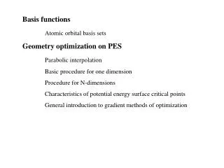
Basis functions Atomic orbital basis sets Geometry optimization on PES Parabolic interpolation
420 likes | 588 Vues
Basis functions Atomic orbital basis sets Geometry optimization on PES Parabolic interpolation Basic procedure for one dimension Procedure for N-dimensions Characteristics of potential energy surface critical points General introduction to gradient methods of optimization.

Basis functions Atomic orbital basis sets Geometry optimization on PES Parabolic interpolation
E N D
Presentation Transcript
Basis functions Atomic orbital basis sets Geometry optimization on PES Parabolic interpolation Basic procedure for one dimension Procedure for N-dimensions Characteristics of potential energy surface critical points General introduction to gradient methods of optimization
Five statements for demythologization: Nº 1.: The term “orbital” is a synonym for the term “One-Electron” Function (OEF) Nº 2.: A single centered OEF is synonymous with “Atomic Orbital”. A multi centered OEF is synonymous with “Molecular Orbital”. Orbital == OEF
Five statements …. • Nº 3.: 3 ways to express a mathematical function: • Explicitly in analytical form • (hydrogen-like AOs) • As a table of numbers • (Hartree-Fock type AOs for numerous atoms) • In the form of an expansion • (expression of an MO in terms of a set of AO)
Five statements …. Nº 4.: The generation of MOs (f-s) from AOs (h-s) is equivalent to the transformation of an N-dimensional vector space where {h}is the original set of non-orthogonal functions. After orthogonalization of the non-orthogonal AO basis set {h} the orthogonal set {c} is rotated to the another orthogonal set{f}. O
Five statements …. Nº 5.: There are certain differences between the shape of numerical Hartree-Fock atomic orbitals (HF-AO), the analytic Slater type orbitals (STO) and the analytic Gaussian type functions (GTF). However , these differences are irrelevant to the final results as the MO can be expanded in terms of any of these complete sets of functions to any desired degree of accuracy. Atomic orbital basis sets
Basis sets Atomic orbital basis sets The generation of MO from AO requires the generation and transformation of the Fock matrix into diagonal form. The elements of the Fock matrix are assembled from integrals in the following fashion: Where the first term is a one-electron integral and the latter terms are two-electron integrals having the following forms.
One-electron integrals: Enormous number of integrals
For the atomic orbital {h} two types of analytic functions are used in molecular computations. 1) Slater-type orbital (STO) or exponential type functions.(ETF). 2) Gaussian-type orbital (GTO) or Gaussian-type function (GTF). The GTF are more popular as it is possible to compute the integrals over Gaussian very quickly, but only relative large N gives accurate results. These AO basis sets need to be optimized for molecular calculation. This may be achieved by minimizing the electronic energy with respect to all orbital exponents.
Sometimes STOs are expanded in terms of GTFs or, in other words, a GTF basis set is contracted to a set of STO. The contraction of a set of three Gaussian-type functions to single Slater function used to be very popular (STO-3G): This means that the total number of integrals to be stored can be reduced by contraction as illustrated bellow:
The contraction of basis set reduces the size of the Fock matrix which will be more manageable to find the solution. In the above case 9 integrals have been evaluated, but only their sum total, that is, a single integral, is stored. The STO-3g basis function is a contracted Gaussian consisting of three primitive Gaussians. Typically, an ab initio basis function consist of a set of primitive Gaussians bundled together with a set of contraction coefficient.
The basic advantage of Gaussian type functions is due to the fact that the product of any two Gaussian is also a Gaussian with its centre on a line between the centres of the two original Gaussian functions. Consequently, all integrals have explicit analytical expressions and may be evaluated rapidly.
A similar theorem does not exist for STO. The principal disadvantages of GTF are their smooth behaviour (lack of cusp) at the nucleus and their too rapid (by rather than by) decrease at large distances. This improper asymptotic behaviour requires the use of a larger number of GTF than STO for equivalent accuracy. However, the much greater speed per integral evaluation in terms of GTF as opposed to STO allows for this greater total number of integrals.
Geometry optimization on PES There are three types of internal motions of molecules: stretch, bend and torsion. The torsion is a periodic motion even if its periodicity low so that it repeats itself only after a 360° rotation. The bending motion usually governs a double-well potential. If the bonds that undergo bending motion are attached to N or O then the barrier to inversion is quite low (from a few to a few tens kcal/mol) but if it involves C then the inversion potential is very high as the inversion would pass through a planar carbon.
If we knew the potential curves that are characteristic to a given molecular system then we could determine the whereabouts of the minimum energy points that in fact correspond to the equilibrium geometry. Unfortunately, these potential functions are not only unknown but they change from molecule to molecule and from bond to bond. However, we do know that they may be approximated, near any of their minima by same quadratic potential, since quadratic and true functions osculate at the minimum.
The quadratic function is the traditional Hooke's law: where G, the second derivative of E with respect to x, is the force constant usually denoted by k The minimum energy point is denoted by Em and xm. For a multi-dimensional problem the generalized Hooke's law may be written as follows:
where is the (x-xm) displacement vector and G, the Hessian matrix, collects all diagonal and off-diagonal or interaction force constants
A schematic illustration of a two-dimensional potential energy surface: E= E(x1,x2) in terms of energy levels contours. Note that the normal coordinates {yi} are different from the internal coordinates {xi}
Molecular geometry optimization involves the finding of the minimum energy (Em) point or in other words locating xlm, x2m; . . .This can most effectively be done by evaluating the gradient vector: and searching for the point where the gradient vector is a zero vector since at the minimum the gradient vanishes Figure 1.2.8—4 ABRA ROSSZ!!!
Characteristics of minima and maxima of a potential energy curve, (Note that g is the gradient, k is the force constant of the potential energy function and l is the index of the critical point in question
Three types of critical points of a potential energy surface and their characteristics in terms of second partial derivatives. (Note that the index (l) of a critical point is the number of negative second derivatives.)
Even though the gradient vector provides a powerful tool in locating the minimum we always carry out the multi-dimensional optimization as a sequence of one-dimensional optimizations. The one-dimensional optimization, however, involves a quadratic or parabolic interpretation. Parabolic interpolation Basic procedure for one-dimension First of all, we must choose an initial point: x0 and a distance: d which lead to three equidistant points (x0 + d), x0, (x0-d). Secondly we need to evaluate E(x) at the three equidistance points leading to three energy values E+, E0 and E- Thirdly, we locate the minimum energy (Em) point which is located at xm. If xm falls within the range x0 - d to x0 + d, and if d is sufficiently small then quit. Of course we want to avoid extrapolation. Alternatively we should get enough (3) equidistant points to bracket xm(1), and predetermine xm(2). This may involve using some of the original points again if xm(1) was close to x0.
Minimum of a parabola A general equation of a parabola may be written as: and the function may be evaluated at three equidistant points (x0 - d), x0, (x0 + d) Expansion gives:
The location of minimum, where x = xm may be achieved by setting the gradient equal to zero It is convenient to introduce the following notations:
This predicted E(xm) is the minimum energy of the quadratic function. This value can be compared to E(xm) calculated from the function. Note also that an estimate of the force constant, the parameter a, is readily obtained. for a maximum a<0 for a minimum a>0
Procedure for N-dimensions First of all, from the start position, one should find the minimum along the first direction(x1). Subsequently, one must cycle through the remaining independent variables, (x2, x3, ...:, xn), fitting parabolas to sets of 3 points in each direction in turn. To reach M1, the best point after the lst cycle through all the parameters. Typical parabolic interpolation optimization of E(xl,x2) (Note that after the start position, mi: end of cycle i, m: true minimum.)
If mi and mi-1 are sufficiently close to each other then quit. Alternatively use Mi as the new start position, and continue. As the optimization progresses, it is desirable to cut down the step size d. While this type of sequential optimization along one internal coordinate before the next one is a working method but it is rather pedestrian. Also, if the variables are coupled, as they very often are, the method is very inefficient.
Characteristics of potential energy surface critical points The force constant or the Hessian matrix is a real symmetric matrix. In diagonal form the diagonal elements are the eigenvalues of the Hessian. Sometime all of these eigenvalues are positive, other times some of them are negative while some of them are positive and other times all of the eigenvalues are negative. This is a general case, for a particular critical point, where the first l diagonal elements are negative and the rest of them are positive. Of course; l may assume values between 0 and n.
The parameter l; the number of negative eigenvalues, is called the index of the particular point. For a minimum l = 0, that is all diagonal elements of Gdiag are positive. For a saddle point, corresponding to a chemical transition state l = 1. For a maximum l = n.
Since the fundamental frequency is related to the square root of the force constant Or , in a multidimensional case , for the m-th diagonal element of Gdiag Therefore, the first l eigenvalues of Gdiag correspond to imaginary frequency. For m>l we obtain At the end of the optimization it is advisable to check the order (l) of the critical point. If l = 0 then we can rest assured that the critical point in our optimization we have converged to is indeed a minimum.
General introduction to gradient methods of optimization Methods for unconstrained optimization of a variables (n dimensions) are designed to produce the answer in a finite number of steps when the function, f(x), is quadratic. It is then hoped that the method will be efficient on more general functions, but especially those with slowly varying second derivatives. For a general function the notation f(x) is used rather than the E(x) specified before. This is done to emphasize that the method is applicable to any routine differentiable function. At the minimum or very close to it the functions have quadratic form, in addition to the constant f(xm ), without a linear term. This function may be written, as follows:
However, some distance away from the minimum at point xk the inclusion of a linear term is advisable as specified by the next equation
The components of the gradient vector g(x) are the first partial derivatives of f(x) In general, the objective function f(x) is or in Dirac notation Where
The gradient of f(x), g(x) is: or where gi(x) is the ith component of |g>. At the extremum of f Letting |xm> be the coordinates of the extremum. Therefore
Substitute for |a>=|g>-G|x> Eq. 1. Which is the Newton (or Newton-Raphson ) equation. Given exact G and |g>, the minimum can be found in one step for a quadratic function. Methods which do not use an exact G often use an approximate matrix H (a positive definite symmetric matrix) such that HG=1 In these cases, the step size is usually written: Eq. 2. where li is to be determined
Note that |x(i+1)> will not necessarily be the extremum desired for any value of li, as H is not exact. Besides if f is not quadratic, eq. 1. is not valid anyways so eq. 2 is always used in practice. Such methods, based on eq. 2., are called quasi-Newton methods.
Steepest descents A very simple optimization method called steepest descents arises from eq. 2. by assuming H is the unit matrix, so that the search direction is always -|g(i)>. A line search is carried out along the direction -|g(i)> to obtain li. This method however, poses some problems. Subsequent search directions tend to be linearly dependent, so only a small subspace of the total space is explored. Directions with large components of |g(i)> are always favoured whereas progress can sometimes be made by searching in orthogonal directions to reach a part of the surface that would allow better progress. Also, the method converges very slowly near the minimum as g(x) is getting smaller in that vicinity.
Summary Start Initial geometry Initial density Current geometry Current density(r) Gradient optimizator HF-SCF Finish or continue Finish or continue Final geometryFinal energyFinal wavefunctionFinal density(r) Flowchart for non-empirical (ab-initio) and semi-empirical (AM1 or PM3) Molecular orbital (MO)computations with geometry optimization