Chapter 6 Inventory Control Models
Chapter 6 Inventory Control Models. Prepared by Lee Revere and John Large. Learning Objectives. Students will be able to: Understand the importance of inventory control and ABC analysis. Use the economic order quantity (EOQ) to determine how much to order.

Chapter 6 Inventory Control Models
E N D
Presentation Transcript
Chapter 6 Inventory Control Models Prepared by Lee Revere and John Large 6-1
Learning Objectives Students will be able to: • Understand the importance of inventory control and ABC analysis. • Use the economic order quantity (EOQ) to determine how much to order. • Compute the reorder point (ROP) in determining when to order more inventory. • Solve inventory problems that allow quantity discounts or non-instantaneous receipt. 6-2
Chapter Learning Objectives continued Students will be able to: • Understand the use of safety stock with known and unknown stockout costs. • Describe the use of material requirements planning in solving dependent-demand inventory problems. • Discuss just-in-time inventory concepts to reduce inventory levels and costs. • Discuss enterprise resource planning systems. 6-3
Chapter Outline 6.1Introduction 6.2Importance of Inventory Control 6.3Inventory Decisions 6.4Economic Order Quantity (EOQ): Determining How Much to Order 6.5Reorder Point: Determining When to Order 6.6EOQ without the Instantaneous Receipt Assumption 6-4
Chapter Outline - continued 6.7Quantity Discount Models 6.8Use of Safety Stock 6.9ABC Analysis 6.10Dependent Demand: The Case for Material Requirements Planning 6.11Just-in-Time Inventory Control 6.12Enterprise Resource Planning 6-5
Inventory as an Important Asset Inventory 40% Other Assets 60% • Inventory can be the most expensive and the most important asset for an organization Inventory as a percentage of total assets 6-6
Inventory Planning and Control - Fig. 6.1 Planning on what Inventory to Stock and How to Acquire It Forecasting Parts/Product Demand Controlling Inventory Levels Feedback Measurements to Revise Plans and Forecasts 6-7
The Inventory Process Suppliers Customers Inventory Storage Raw Materials Finished Goods Fabrication and Assembly Work in Process Inventory Processing 6-8
Importance of Inventory Control Five Functions of Inventory • Decoupling • Storing resources • Responding to irregular supply and demand • Taking advantage of quantity discounts • Avoiding stockouts and shortages 6-9
Inventory Decisions Two fundamental decisions in controlling inventory: • How much to order • When to order Overall goal is to minimize total inventory cost 6-10
Inventory Costs • Cost of the items • Cost of ordering • Cost of carrying, or holding inventory • Cost of safety stock and stockouts 6-11
Ordering Costs • Developing and sending purchase orders • Processing and inspecting incoming inventory • Bill paying • Inventory inquiries • Utilities, phone bills, etc., for the purchasing department • Salaries/wages for purchasing department employees • Supplies (e.g., forms and paper) for the purchasing department 6-12
Carrying Costs • Cost of capital • Taxes • Insurance • Spoilage • Theft • Obsolescence • Salaries/wages for warehouse employees • Utilities/building costs for the warehouse • Supplies (e.g., forms, paper) for the warehouse 6-13
Inventory Usage Over Time - Fig. 6.2 Sawtooth Inventory Curve 6-14
Costs as Functions of Order Quantity - Fig. 6.3 Annual Cost Carrying (holding) Cost Curve Total Cost Curve Minimum Cost Ordering (set-up) Cost Curve Q* Order Quantity View #1 6-15
Costs as Functions of Order Quantity - Fig. 6.3 View #2 Total Cost Minimum Cost Carry Cost Order Cost Optimal Quantity 6-16
EOQ : Basic Assumptions • Demand is known and constant. • Lead time is known and constant. • Receipt of inventory is instantaneous. • Quantity discounts are not possible. • The only variable costs: set-up or placing an order, and holding or storing inventory over time. • Stockouts can be completely avoided if orders are placed at the appropriate time. 6-17
Steps in Finding the Optimum Inventory • Develop an expression for the ordering cost. • Develop and expression for the carrying cost. • Set the ordering cost equal to the carrying cost. • Solve this equation for the optimal order quantity, Q*. 6-18
Developing the EOQ • Annual ordering cost: • Annual holding or carrying cost: • Total inventory cost: 6-19
Setting the Equations Equal to Solve for Q* Q D C = + C C h t 2 o Q D Q = C C o h Q 2 2 2 D D Q2 = C C o o C C Q* = h h 6-20
Per Unit vs. Percentage Carrying Cost • Typically, carrying cost, Ch, is stated in • per unit $ cost • per year • Sometimes, an annual Interest rate, I, is cited and Ch must be calculated • I multiplied by C (unit cost) • IC then replaces Ch 6-21
EOQ 2DC 2DC o o C h * = Q IC Per Unit Carrying Cost: * = Q Denominator Change Percentage Carrying Cost: 6-22
Inputs and Outputs of the EOQ Model Input Values Output Values Economic Order Quantity (EOQ) Annual Demand (D) Avg. Inventory (Q/2) Ordering Cost (Co) EOQ Models # of Orders (D/Q) Carrying Cost (Ch) Lead Time (L) Cycle Time (Q/D*360) Reorder Point (ROP) Demand Per Day (d) 6-23
The Reorder Point (ROP) Curve - Fig. 6.4 Q* Slope = Units/Day = d ROP (Units) Inventory Level (Units) L Lead Time (Days) ROP = (Demand per day) x (Lead time for a new order, in days) = d x L 6-24
Inventory Control and the Production Process Suspension of the Instantaneous Receipt Assumption Production Portion of Cycle (t) = Q/p Maximum Inventory Level Q* Inventory Level Demand Portion of Cycle Demand Portion of Cycle Time Production Run Model Figure 6.5 6-25
Production Quantity EOQ • Annual Carrying Cost: • Annual Setup or Ordering Cost: • Setup Cost: • Ordering Costs: Q d - ( 1 ) C h 2 p D C s Q D C o Q 6-26
Production Quantity EOQ 2DC * = Q s p ö æ _ d ÷ ç C 1 ÷ ç p h ø è If production is not the cause of delayed receipts, use the same model but replace Cs with Co 6-27
Brown Manufacturing Example • Annual demand (D) = 10,000 units • Setup cost (Cs) = $100 • Carrying cost (Ch) = $0.50 per unit per year • Production rate (p) = 80 units daily • Demand rate (d) = 60 units daily • Refrigeration operational days = 167 days per year 6-28
Brown Manufacturing Example continued • How many refrigeration units should Brown produce in each batch? • i.e., What is Qp*? • How long should the production cycle last ? • i.e., What is Q/p? 6-29
Brown Manufacturing Example continued 2DC * = Q s p ö æ _ d ÷ ç C 1 ÷ ç p h ø è * * Q Q p p æ ö ç ÷ ç ÷ è ø • What is Qp*? 2(10,000)(100) = 60 _ 1 (0.5) 80 = 4,000 units 6-30
Brown Manufacturing Example continued * Q p = 4,000 units • How long should the production cycle last ? What is t (Q/p)? p = 80 units per day t = Q/p = 4,000/80 = 50 days Production runs will cover 50 days and produce 4,000 units 6-31
Quantity Discount Models • Object is to Minimize total inventory costs; includes material costs • Material costs relevant in total cost: • TC = DC + D/Q(Co) + Q/2(Ch) where • D = unit annual demand • C = unit cost • Co = each order cost • Ch = carrying cost per unit per year IC must be used in place of Ch in decision-making 6-32
Steps for Solving Quantity Discount 2DC o * = Q IC • Compute EOQ for each discount price: • If EOQ < discount minimum level, make Q = minimum. • For each EOQ, compute total cost: TC = DC + D/Q(Co) + Q/2(Ch) • Choose the lowest cost quantity from all levels. 6-33
Quantity Discount Models – Table 6.3 Text example: Quantity Discount Schedule Table 6.3 • Material cost: • Total material cost is affected by the • Discount (%) • Unit cost if first $5.00, then $4.80, • and finally $4.75 6-34
Quantity Discount Models - Fig. 6.6 Total Cost Curves for each of the 3 discount plans Figure 6.6 6-35
Quantity Discount Steps – A Review 1. Calculate Q for each discount. 2. Adjust Q upward if quantity is too low for discount. 3. Compute total cost for each discount. 4. Select Q with the the lowest total cost. 6-36
The Use of Safety Stock • Stockouts occur when there are uncertainties with: • Demand • Lead time • Safety stock is extra stock on hand to avoid stockouts • ROP is adjusted to implement safety stock policy: • ROP = d*L + SS • d = average daily demand • L = average lead time, time for an order to be delivered • SS = safety stock 6-37
The Use of Safety Stock Fig. 6.7 Inventory on Hand 0 Time Stockout Inventory on Hand Stockout is avoided Safety Stock 0 Time 6-38
The Use of Safety Stock and ROP • Known stockout costs: • Given probability of demand, find total cost for each safety stock alternative • Unknown stockout costs: • Set service level; use normal distribution 6-39
Known Stockout Costs • ABCO example: Table 6.5 Initial calculations: ROP = 50 (d*L) Ch = $5 Css = $40/ unit (stockout cost) D/Q = 6 times per year 6-40
Known Stockout Costs continued • ABCO example: Table 6.6 Calculation the EMV (expected monetary value) for each ROP alternative 6-41
Known Stockout Costs continued • ABCO example: • Calculations for a given ROP, N: • Being Short: D(S) = (N-S)* Css *D/Q, • where S = demand during lead time • Being Over: D(O) = (D-O)* Ch • where O = demand under ROP • Calculations for an ROP of 40: • Being Over • D(30) = (40-30)*$5 = $50 • D(40) = $0 • Being Short • D(50) = (50-40)*$40*6 = $2,400 • D(60) = (60-40)*$40*6 = $4,800 • D(70) = (70-40)*$40*6 = $7,200 6-42
Known Stockout Costs continued • ABCO example: Last step for ROP = 40 is to calculate the EMV: EMV = S P(D) * Cost of Being Short/Over EMV(40) = 0.20*$50 + 0.20*$0 + 0.30*$2,400 + 0.20*$4,800 + 0.10*$7,200 = $2,410 6-43
Unknown Stockout Costs • When stockout costs are not quantifiable or not applicable: • Use a service level to determine safety stock level. • Service Stock: the % of time an item is out of stock. Service Level = 1 – P(Stockout) Or P(Stockout) = 1 – Service Level 6-44
Unknown Stockout Costs continued Hinsdale Company example: • Lead time demand ~N(350, 10) • where m = 350, s = 10 • Desired Policy: P(Stockout) = 5% Therefore, service level = 95% Visualization of Desired Inventory Policy: Figure 6.9 6-45
Unknown Stockout Costs continued Hinsdale Company example: X = m + Safety Stock (SS) SS = X – m = Zs Z = = Figure 6.9 X-m SS s s 6-46
Unknown Stockout Costs continued Hinsdale Company example: Find Z using a Normal table, like in Appendix A: Z = 1.65 for a 5% right tail Rewrite equation: Z = 1.65 = = Solving for SS yields 16.5, or 17, units. Therefore, ROP = 350 + 17 = 367 SS SS s 10 6-47
Service Level versus Carrying Costs The following curve depicts the tradeoff between carrying costs and service level for the previous example such dramatic tradeoffs exist for all similar problems Figure 6.10 6-48
Summary of ABC Analysis Table 6.6 Are Complex Quantitative Control Techniques Used? Inventory Group Dollar Usage (%) Inventory Items (%) Yes In some cases No A B C 70 20 10 10 20 70 • Group A Items - Critical • Group B Items - Important • Group C Items - Not That Important 6-49
ABC Inventory Analysis 100 90 80 70 60 50 40 30 20 10 0 A Items Percent of Annual Dollar Usage B Items C Items 1 2 3 4 5 6 7 8 9 10 Percent of Inventory Items 6-50