Inventory Control Models: Learning Economic Order Quantity (EOQ)
Learn how to calculate optimal order quantities to minimize inventory costs using the Economic Production Lot (EPL) model in Excel. Understand the types of inventory, reasons for holding inventory, and calculate costs with a real-world production scenario.


Inventory Control Models: Learning Economic Order Quantity (EOQ)
E N D
Presentation Transcript
Inventory control models EPL Model
Learning objective • After this class the students should be able to: • calculate the order quantity that minimize the total cost inventory, based on the EPL model and • analyze the implication of this model using what-if through the Excel software.
Time management • The expected time to deliver this module is 50 minutes. 30 minutes are reserved for team practices and exercises and 20 minutes for lecture.
Inventory & inventory system • Inventory is the set of items that an organization holds for later use by the organization. An inventory system is a set of policies that monitors and controls inventory. It determines how much of each item should be kept, when low items should be replenished, and how many items should be ordered or made when replenishment is needed.
Basic types of inventory • independent demand, • dependent demand, and • supplies.
Independent Demand • Independent demanditems are those items that we sell to customers. • Dependent demanditems are those items whose demand is determined by other items. Demand for a car translates into demand for four tires, one engine, one transmission, and so on. The items used in the production of that car (the independent demand item) are the dependent demand items. • Supplies are items such as copier paper, cleaning materials, and pens that are not used directly in the production of independent demand items
Why hold Inventory • Each team is invited to discuss for 10 minutes about what they figure out to be the reasons that the organizations maintain inventory. At the and, they have to present a list of their supposed reasons.
Five reasons • To decouple workcenters; • To meet variations in demand; • To allow flexible production schedules; • As a safeguard against variations in delivery time; and • To get a lower price.
The cost of Inventory • Holding costs; • Setup costs; • Ordering costs; and • Shortage costs.
Notation • D= Demand rate (in units per year). • c = Unit production cost, not counting setup or inventory costs (in dollars per unit). • A = Constant setup (ordering) cost to produce (purchase) a lot (in dollars). • h = Holding cost • Q = Lot size (in units); this is the decision variable
Economic Lot Size Production Model • We use the same notation and assumptions of the EOQ model, but now P ( that not is instantaneous) designates the production rate, and t designates the time needed to produce the lot. Then, Q= P x t
The problem • Beth Krider, Manager of Production for Zap Electronics, is making production plans for microphones for portable recorders. The rate of production (P) is 4,000 microphones per month, and the (D) demand rate is 1,000 microphones per month. The cost of each microphone is $6.75, and the inventory holding percent is 0.2. • She is wondering whether this lot size gives the lowest cost.
Cumulative production and Demand 4,000 microphones were made in January, and in February, March, and April, no microphones were produced. 1,000 microphones were sold in January, resulting in an inventory of 3,000 microphones on February 1. The inventory is used up in February, March, and April, so that on April 30 there is no inventory. Then the whole cycle repeats.
Monthly inventory of microphones The maximum inventory is 3,000 microphones, and the average inventory is 3,000/2 = 1,500 microphones. Note the similarity between this problem and the EOQ problem we have already shown
Now A, the ordering cost, designates the setup cost for producing a lot of the microphones. • P designates the production rate, and t designates the time needed to produce the lot.
Average Inventory Level • The maximum inventory is • The average inventory is where
The Factor F • Demand rate (D) must be less than or equal to the production rate (P). If D = P, production just meets the demand. In this case, the factor is 0, and so is the inventory. If the production rate is very large compared to the demand, D/P is very small. In such cases, the factor is near 1 and the average inventory is Q/2, the same as in the EOQ problem. The straight line shows how the factor depends on the value of D/P.
The Costs • Annual holding cost Where C=cost of each microphone and i =interest rate • Annual setup cost = D/Q x A
The total cost • To carry out the calculations, we need the other parameters of the problem. • Cost of each microphone: C = 6.75 • Percent of holding cost: i = 20% • Setup cost: A = $28 Then, • Annual holding cost = 4,000 x 3/4 x 6.75 x 0.2/2 = $2,025 • Annual setup cost = 12,000/4,000 x 28 = $84 • Annual total cost = $2,109
The model Appling the conditions for optimization, we find the optimal value for order quantity and Cost
Conclusion • We calculated the optimal production lot size and the costs and found that Q* = 814.68, and the total cost is $824.87. • This is $1.284.13 less than Beth's solution of ordering 4,000 microphones three times a year.
What-if • Each team is invited to built a model in the Excel software and develop what-if analysis (10) minutes
Open excel file What-if
Reference • Operations Analysis Using Excel. Weida; Richardson and Vazsony, Duxbury, 2001,Chapter 6.