Interfacing Methods and Circuits
Interfacing Methods and Circuits. Chapter 11. Introduction. A sensor/actuator can rarely operate on its own. Exceptions exist (bimetal sensors) Often a circuit of some sort is involved. can be as simple as adding a power source or a transformer


Interfacing Methods and Circuits
E N D
Presentation Transcript
Interfacing Methods and Circuits Chapter 11
Introduction • A sensor/actuator can rarely operate on its own. • Exceptions exist (bimetal sensors) • Often a circuit of some sort is involved. • can be as simple as adding a power source or a transformer • can involve amplification, impedance matching, signal conditioning and other such functions. • often, a digital output is required or desirable so that an A/D may be needed • The same considerations apply to actuators
Introduction • The considerations of interfacing should be part of the process of selecting a device for a particular application since this can simplify the process considerably. • Example: if a digital device exists it would be wasteful to select an equivalent analog device and add the required circuitry to convert its output to a digital format. • The likely outcome is a more cumbersome, expensive system which may take more time to produce. • Alternative sensing strategies and alternative sensors should always be considered before settling on a particular solution
Introduction • Many types of sensors and actuators based on very different principles • There are commonalities between them in terms of interfacing requirements • Most sensors’ outputs are electric (voltage, current, resistance) • These can be measured directly after proper signal conditioning and, perhaps, amplification. • If the output is a capacitance or an inductance - require additional circuitry such as oscillators
Introduction • There is a large range of signal levels in sensors. • A thermocouple’s output is of the order of microvolts • An LVDT may easily produce 5V AC. • A piezoelectric actuator may require a few hundred volts to operate (very little current) • A solenoid valve operates at perhaps 12-24V with currents that may exceed a few amperes. • How does one measure/generate/interface these signals?
Introduction • The circuitry required to drive and to interface them to, say a microprocessor are vastly different • Require special attention on the part of the engineer. • Must consider such issues as response (electrical and mechanical), spans and power dissipation as well as power quality and availability. • Example: Systems connected to the grid and cordless systems have different requirements and considerations in terms of operation and safety.
Purpose • Discuss general issues associated with interfacing • Outline general interfacing circuits the engineer is likely to be exposed to. • No general discussion however can prepare one for all eventualities • It should be recognized that there are both exceptions to the rules and extensions to the methods discussed here.
Purpose • Example: an A/D is a simple – if not inexpensive – method of digitizing a signal for the purpose of interfacing • This approach however may not be necessary and too expensive in some cases. • Suppose the hall element senses the teeth on a gear. • The signal from the hall element is an ac voltage - only the peaks are necessary to sense the teeth. • In this case a simple peak detector may be adequate. • An A/D converter will not provide any additional benefit and is a much more complex and expensive solution. • On the other hand, if a microprocessor is used and an A/D is available internally, it may be acceptable to use it for this purpose
Content • Operational amplifiers and power amplifiers • A/D and D/A conversion circuits • Bridge circuits • Data transmission • Excitation circuits • Noise and interference
Amplifiers • An amplifier is a device that amplifies a signal – almost always a voltage • The low voltage output of a sensor, say of a thermocouple, may be amplified to a level required by a controller or a display. • Amplification may be quite large – sometimes of the order of 106 or it may be quite small or even smaller than one, depending on the need of the sensor.
Amplifiers • Amplifiers can also be used for impedance matching purposes even when no amplification is needed • May be used for the sole purpose of signal conditioning, signal translation or for isolation • Power amplifiers, which usually connect to actuators, serve similar purposes beyond providing the power necessary to drive the actuator. • Amplifiers can be very simple – a transistor with its associated biasing network or may involve many amplification stages of varying complexity. • Amplifiers are sometimes incorporated in the sensor
Amplifiers • We will use the operational amplifier as the basic building block for amplification. • Operational amplifiers are basic devices and may be viewed as components. • An engineer, especially when interfacing sensors is not likely to dwell into the design of electronic circuits below the level of operational amplifiers. • Although there are instances where this may be done to great advantage, op-amps are almost always a better, less expensive and higher performance choice. • Same idea for power amplifiers
Operational Amplifiers • Operational amplifier is a fairly complex electronic circuit but: • It is based on the idea of the differential voltage amplifier shown in Figure 11.1. • Based on simple transistors, • The output is a function of the difference between the two inputs. • Assuming the output to be zero when both inputs are at zero potential, the operation is as follows:
Operational amplifier • When the voltage on the base of Q1 increases, its bias increases while that on Q2 decreases because of the common emitter resistance. • Q1 conducts more than Q2 and the output is positive with respect to ground. • If the sequence is inverted, the opposite occurs. • If, both inputs increase or decrease equally, there will be no change in output.
Operational amplifier • An operational amplifier is much more complex than this but operates on the same principle. • It contains additional circuitry (such as temperature and drift compensation, output amplifiers, etc.) • These are of no interest to us other than the fact that they affect the specifications of the op-amp. • There are also various modifications to op-amps that allow them to operate under certain conditions or to perform specific functions.
Operational amplifier • Some are “low noise” devices • Others can operate from a single polarity source. • If the input transistors are replaced with FETs, the input impedance increases considerably requiring even lower input currents from sensors • These are important but are variations of the basic circuit. • We will consider it as a simple block shown in Figure 11.2 and discuss its general properties based on this diagram
Op-Amps - properties • Differential voltage gain: the amplification of the op-amp of the difference between the two inputs: • Also called the open loop gain • In a good amplifier it should be as high as possible. • Gains of 106 or higher are common. • An ideal amplifier is said to have infinite gain.
Op-Amps - properties • Common-mode voltage gain. • By virtue of the differential nature of the amplifier, this gain should be zero. • Practical amplifiers may have a small common mode gain because of the mismatch between the two channels but this should be small. • Common mode voltage gain is indicated as Acm. • The concept is shown in Figure 11.3.
Op-amps - properties • More common to specify the term Common Mode Rejection Ratio (CMRR) • CMRR is the ratio between Ad and Acm: In an ideal amplifier this is infinite. A good amplifier will have a CMRR that is very high
Op-amps - properties • Bandwidth: the range of frequencies that can be amplified. • Usually the amplifier operates down to dc and has a flat response up to a maximum frequency at which output power is down by 3dB. • An ideal amplifier will have an infinite bandwidth. • The open gain bandwidth of a practical amplifier is fairly low • A more important quantity is the bandwidth at the actual gain.
Op-amps - properties • This may be seen in Figure 11.4 • The lower the gain, the higher the bandwidth. • Data sheets therefore cite what is called the gain-bandwidth product. • This indicates the frequency at which the gain drops to one and is also called the unity gain frequency. • In Figure 11.4: • BW (open loop) is 2.5 kHz • Unity Gain Frequency is 5 MHz
Op-amps - properties • Slew Rate: the rate of change of the output in response to a change in input, given in V/s. • If a signal at the input changes faster than the slew rate, the output will lag behind it and a distorted signal will be obtained. • This limits the usable frequency range of the amplifier. • For example, an ideal square wave will have a rising and dropping slope at the output defined by the slew rate.
Op-amps - properties • Input impedance: the impedance seen by the sensor when connected to the op-amp. • Typically this impedance is high (ideally infinite) • It varies with frequency. • Typical impedances for conventional amplifiers is at least 1 M but it can be of the order of hundreds of M for FET input amplifiers. • This impedance defines the current needed to drive the amplifier and hence the load it represents to the sensor.
Op-amps - properties • Output impedance: the impedance seen by the load. • Ideally this should be zero since then the output voltage of the amplifier does not vary with the load • In practice it is finite and depends on gain. • Usually, output impedance is given for open loop whereas at lower gains the impedance is lower. • A good amplifier will have an output resistance lower than 1.
Op-amps - properties • Temperature and noise refer to variations of output with temperature and noise characteristics of the device respectively. • These are provided by the data sheet for the op-amp and are usually very small. • For low signals, noise can be important while temperature drift, if unacceptable must be compensated for through external circuits.
Op-amps - properties • Power requirements. The classical op-amp is built so that its output can swing between ±Vcc • Dual supply operation is common in op-amps • The limits can be as low as ±3V (or lower) and as high as ±35V (sometimes higher). • Many op-amps are designed for single supply operation of less than 3V and some can be used in single supply or dual supply modes.
Op-amps - properties • Current through the amplifier is an important consideration, especially the quiescent current (no load) • Gives a good indication of power needed to drive it. • Particularly important in battery operated devices. The current under load will depend on the application but it is usually fairly small – a few mA. • In selection of a power supply for op-amps, care should be taken with the noise that the power supply can inject into the amplifier. • The effect of the power supply on the amplifier is specified through the power supply rejection ratio (PSRR) of the specific amplifier.
Op-amps - data sheets • The 741 op-amp is an older, general purpose amplifier. • It is a fairly low performance device but is characteristic of the low-end amplifiers. • Very common and quite suitable for many applications. LM741.PDF
Op-amps - data sheets • The TLC27L2C is a dual, low power op-amp, suited for battery operated devices • Part of a series of amplifiers using FETs as input transistors TLC27L2C
Inverting and noninverting amplifiers • Performance of the amplifier depends on how it is used and, in particular on the gain of the amplifier. • In practical circuits, the open loop gain is not useful and a specific gain must be established. • For example, we might have a 50mV output (maximum) from a sensor and require this output to be amplified, say by 100 to obtain 5V (maximum) for connection to an A/D. • This can be done with one of the two basic circuits shown in Figure 11.5 by establishing a means of negative feedback to reduce the gain
Inverting op-amp • The output is inverted with respect to the input (180 out of phase). • The feedback resistor, Rf, feeds back some of this output to the input, effectively reducing the gain. • The gain of the amplifier is now given as: In the case shown here this is exactly –10
Inverting op-amp • The input impedance of the amplifier is given as Here it is equal to 1 k. If a higher resistance is needed, larger resistances might be needed Or, perhaps, a different amplifier will be needed (noninverting amplifier)
Inverting op-amp • The output impedance of the amplifier is given as AOL is the open loop gain as listed on the data sheet Open loop gain is the open loop gain at the frequency at which the device is operated
Inverting op-amp • Example, for the LM741 amplifier, the open loop output impedance is 75W and the open loop gain at 1 kHz is 1000. This gives an output impedance of: The bandwidth is also influenced by the feedback:
Non-inverting amplifier • The non-inverting amplifier gain is: For the circuit shown, this is 11 The gain is slightly larger than for the noninverting amplifier for the same values of R. The main difference however is in input impedance.
Non-inverting amplifier • Input impedance is: • Rop is the input impedance of the op-amp as given in the spec sheet • Aol is the open loop gain of the amplifier. • Assuming an open loop impedance of 1 M (modest value) and an open loop gain of 106, we get an input impedance of 1011. (almost ideal)
Non-inverting amplifier • The output impedance and bandwidth are the same as for the inverting amplifier. • The main reason to use a noninverting amplifier is that its input impedance is very large making it almost ideal for many sensors. • There are other properties that need to be considered for proper design such as output current and load resistance but these will be omitted here for the sake of brevity.
The voltage follower • The feedback resistor in the noninverting amplifier is set to zero • The circuit in Figure 11.6 is obtained. • The gain is one. • This circuit does not amplify. • Why use it?
Voltage follower The input impedance now is very large and equal to: The output impedance is very small and equal to:
Voltage follower • The value of the voltage follower is to serve in impedance matching. • One can use this circuit to connect, say, a capacitive sensor or an electret microphone. • If amplification is necessary, the voltage follower may be followed by an inverting or noninverting amplifier
Instrumentation amplifier • The instrumentation amplifier is a modified op-amp • Its gain is finite and both inputs are available to signals. • These amplifiers are available as single devices • To understand how they operate, one should view them as being made of three op-amps (it is possible to make them with two op-amps or even with a single op-amp), as shown in Figure 11.7.
Instrumentation amplifier • The gain of an amplifier of this type is: In a commercial instrumentation amplifier all resistances are internal and produce a gain usually around 100. Ra is external and can be set by the user to obtain the gain required.