PHOENICS
Computer Simulation of Fluid Flow, Heat Flow, Chemical Reactions and Stress in Solids. CHAM. PHOENICS. Application of Environment Spatial Information System. Minkasheva Alena Thermal Fluid Engineering Lab. Department of Mechanical Engineering Kangwon National University 2007.05.04

PHOENICS
E N D
Presentation Transcript
Computer Simulation of Fluid Flow, Heat Flow, Chemical Reactions and Stress in Solids. CHAM PHOENICS Application of Environment Spatial Information System Minkasheva Alena Thermal Fluid Engineering Lab. Department of Mechanical Engineering Kangwon National University 2007.05.04 Part 1
1 Contents • Chapter 1. PHOENICS Overview • 1. What PHOENICS is • 2.The components of PHOENICS • 2.1 The main functions of PHOENICS • 2.2 The structure of PHOENICS • 2.3 The inter-communication files • 2.4 How the problem is defined • 2.5 How PHOENICS makes the predictions • 2.6 How the results are displayed • 2.7 PHOENICS options • 3. Physical content of PHOENICS • 4. Mathematical features of PHOENICS • 4.1 Variables
2 Contents • 4.2 Storage • 4.3 Grids • 4.4 The Balance Equation • 4.5 Auxiliary Equations • 4.6 Solution of Equations • 4.7 Boundary Conditions • 5. Simulation of multi-phase flow in PHOENICS • 6. Turbulence models in PHOENICS • 7. Radiative-heat-transfer models in PHOENICS • 8. Chemical-reaction processes in PHOENICS • 9. Simultaneous solid-stress analysis • 10. Body-fitting in PHOENICS • 11. PHOENICS Application
3 Contents • Chapter 2. The Virtual-Reality Interface • 1. VR-Editor • 1.1 What the Virtual-Reality Editor creates • 1.2 Domain Attributes Menu • 1.3 Object Management Panel • 1.4 Object Types and Attributes • 1.5 The VR Editor Control Panel • 2. VR Viewer • Chapter 3. PHOENICS Application Example • “Simulation ofContaminant Flow” • Pre-Processor VR-Editor • Main Solver Earth • Post-Processor VR-Viewer
Chapter 1 PHOENICS Overview
1 1. What PHOENICS is • PHOENICS is a general-purpose software package which predicts quantitatively: ▪ how fluids (air, water, steam, oil, blood, etc) flow in and around: ᆞ enginesᆞ process equipmentᆞ buildings ᆞ human beings ᆞ lakes, river and oceans, and so on ▪ the associated changes of chemical and physical composition ▪ the associated stresses in the immersed solids • “PHOENICS” - Parabolic Hyperbolic Or Elliptic Numerical Integration Code Series
2 1. What PHOENICS is • PHOENICS is employed by: ▪ scientists for interpreting their experimental observations ▪ engineers for the design of aircraft and other vehicles, and of equipment which produces power or which processes materials ▪ architects for the design of buildings ▪ environmental specialists for the prediction, and if possible control, of environmental impact and hazards ▪ teachers and students for the study of fluid dynamics, heat transfer, combustion and related disciplines • PHOENICS is a “CFD code”Computational Fluid Dynamics software
2. The Components of PHOENICS 2.1 The main functions of PHOENICS •PHOENICS performs three main functions: 1. Problem definition (pre-processing) in which the user prescribes the situation to be simulated and the questions which are to be answered 2. Simulation (data-processing)by means of computation, of what the laws of science imply in the prescribed circumstances 3. Presentation (post-processing)of the results of the computation, by way of graphical displays, tables of numbers, and other means
1 2.2 The structure of PHOENICS
2 2.2 The structure of PHOENICS • PHOENICS has a ‘planetary’ arrangement, with a central core of subroutines called EARTH, and a SATELLITE program, which accepts inputs through the Virtual Reality (VR) interface corresponded to a particular flow simulation. • EARTH and SATELLITE are distinct programs. • SATELLITE is a data-preparation program; it writes a data file which EARTH reads. • PHOENICS users work mainly with SATELLITE, but they can access EARTH also in controlled ways. • GROUND is the EARTH subroutine which users access when incorporating special features of their own.
2.3 The inter-communication files • Files which are used for communication between modules ▪Q1, the user-readable input-data file, which is written in PIL, the PHOENICS Input Language, and is the main expression of what the user wishes to achieve. ▪ EARDAT, an ASCII file which expresses in EARTH-understandable form what the user has prescribed by way of Q1. ▪PHI, which is written by EARTH in accordance with a format which enables PHOTON, AUTOPLOT and the Viewer to display the results of the computation graphically. ▪RESULT, which is an ASCII file expressing the results in tabular and line-printer-plot form
2.4 How the problem is defined ▪geometryshapes, sizes and positions of objects and intervening spaces; ▪materialsthermodynamic, transport and other properties of the fluids and solids involved ▪processesfor example: whether the materials are inert or reactive;whether turbulence is to be simulated and if so by what model;whether temperatures are to be computed in both fluids and solids;whether stresses in solids are to be computed ▪gridthe manner and fineness of the sub-division of space and time, what is called the "discretization" ▪other numerical (non-physical) parametersaffecting the speed, accuracy and economy of the simulation •Problem definition involves making statements about:
2.5 How PHOENICS makes the predictions •PHOENICS simulates physical phenomena by: ▪expressing the relevant laws of physics and chemistry, and the "models" which supplement them, in the form of equations linking the values of pressure, temperature, concentration, etc which prevail at clusters of points distributed through space and time ▪locating these point-clusters (which constitute the computational grid) sufficiently close to each other to represent adequately the continuity of actual objects and fluids ▪solving the equations by systematic, iterative, error-reduction methods, the progress of which is made visible on the VDU screen ▪terminating when the errors have been sufficiently reduced affecting the speed, accuracy and economy of the simulation
2.6 How the results are displayed •PHOENICS can display the results of its flow simulations in a wide variety of forms ▪ It has its own stand-alone graphics package called PHOTON; and it can also export results to such third-party packages as TECPLOT, AVS, and FEMVIEW. ▪PHOENICS can also take the results of its flow predictions back into the same VIRTUAL-REALITY environment as is used for setting up the problem at the start. ▪Numerical results are provided, in the RESULT file. This, when the appropriate commands in the Q1 file, can provide either sparse or voluminous information
2.7 PHOENICS options: • Advanced-multiphase • Body-fitted-coordinate • Advanced-chemistry • GENTRA (particle tracking) • Multi-block and fine-grid-embedding • Multi-fluid • Advanced-algorithms • MIGAL, the multi-grid solver • PLANT fortranizer • Advanced-radiation • Simultaneous-solid-stress • Advanced-turbulence • Two-phase
1 3. Physical content of PHOENICS • PHOENICS simulates flow phenomena which are: • laminar or turbulent • compressible or incompressible • steady or unsteady • chemically inert or reactive • single- or multi-phase • in respect of thermal radiation: • - transparent • - participating by way of absorption and emission • - participating by way of scattering
2 3. Physical content of PHOENICS •The space in which the fluid flows may be: • empty of solids, or • wholly or partially filled by finely-divided solids at rest (as in 'porous-medium' flows), or • partially occupied by solids which are not small compared with the size of the local computational cells The solids may interact thermally with the solids. Such immersed solids can also participate in radiative heat transfer. The thermally and mechanically-induced stresses and strains in the immersed solids can also be computed by PHOENICS. The thermodynamic, transport (including radiative), chemical and other properties of the fluids and solids may be of arbitrary complexity.
4. Mathematical features 1 4.1 Variables •Variables may be thought of as being: • dependent - the subject of a conservation equation • auxiliary - constant, or derived from an algebraic expression •Dependent: • Scalars: • - Pressure • - Temperature • - Enthalpy • - Mass fractions • - Volume fractions • - Turbulence quantities • - Various potentials • Vectors: • - Velocity resolutes • - Radiation fluxes • - Displacements
2 4.1 Variables •Auxiliary: • Vectors: • - Various non-isotropic properties • - Gravity forces • - Other body forces • Scalars: • - Density • - Viscosity • - Conductivity • - Diffusivity • - Specific heat • - Thermal expansion coefficient • - Inter-fluid transport • - Absorptivity • - Compressibility
3 4.1 Variables •The quantities defining the problem geometry can also be divided into scalar and vector categories: • Geometric: • Scalars: • - Cell volumes • - Volume porosity factors • - Inter-fluid surface area per unit volume • Vectors: • - Cell center coordinates • - Cell corner coordinates • - Center to center distances • - Cell surface areas • - Cell area porosities
4.2 Storage • Scalars - These are stored at the center points of six-sided cells, with values supposed to be typical of the whole cell. • Vectors - These are stored at the center points of the six cell faces •NomenclatureA compass-point notation: P = Cell center N,S,E,W,H,L = Neighbour-cell centers S → N = Positive IY W → E = Positive IX L → H = Positive IZ T = Cell center at previous time step An array of cells with the same IZ is referred to as a SLAB
4.3 Grids •Storage locations Vector quantities are computed by reference to cells which are staggered with respect to the scalar cells 3 velocities and 1 scalar share the same cell index (IX,IY,IZ). Any scalar or vector quantity can only be referenced by a unique (IX,IY,IZ) index
4.3 Grids •Types of Grid PHOENICS grids are structured - cells are topologically Cartesian brick elements •PHOENICS grids may be : - Cartesian - Cylindrical-polar - Body fitted i.e. arbitrarily curvi-linear, orthogonal or non-orthogonal The grid distribution can be non-uniform in all coordinate directions •For cylindrical-polar coordinates: - X (or I) is always the angular direction - Y (or J) is always the radial direction - Z (or K) is always the axial direction
4.4 The Balance Equation •Basic form The basic balance, or conservation equation is just: Outflow from cell - Inflow into cell = Net source within cell •The equations solved by PHOENICS are those which express the balances of: • mass • momentum • energy • material (ie chemical species) • other conserved entities (e.g. electrical charge) • over discrete elements of space and time, i.e. 'finite volumes' known as 'cells'
4.4 The Balance Equation •Terms The terms appearing in the balance equation are: - Convection (i.e., directed mass flow) - Diffusion (i.e., random motion of electrons, molecules or larger structures e.g., eddies) - Time variation (i.e., directed motion from past to present - accumulation within a cell) - Sources (e.g., pressure gradient or body force for momentum, chemical reaction for energy or chemical species)
4.4 The Balance Equation •The Generalized Form The single phase conservation equation solved by PHOENICS can be written as: where: - the variable in question - density - vector velocity - the diffusive exchange coefficient for - the source term
4.4 The Balance Equation •Particular Forms Enthalpy Momentum Continuity where , are the turbulent and laminar viscosities, , are the turbulent and laminar Prandtl/Schmidt Numbers
4.4 The Balance Equation •Numerical solution • The balance equations cannot be solved numerically in differential form. Hence, PHOENICS solves a finite-volume formulation of the balance equation. • The FVE's are obtained by integrating the differential equation over the cell volume. • Interpolation assumptions are required to obtain scalar values at cell faces and vector quantities at cell centers. • No Taylor series expansion or variational principle is used
4.4 The Balance Equation •Finite Volume Form After integration, the FVE has the form: where: The neighbour links, the a's, have the form convection diffusion transient
4.4 The Balance Equation •Correction Form The equation is cast into correction form before solution. In correction form, the sources are replaced by the errors in the real equation, and the coefficients may be only approximate. The corrections tend to zero as convergence is approached, reducing the possibility of round-off errors affecting the solution. The neighbor links: - Increase with inflow velocity, cell area, fluid density and transport coefficient - Decrease with internodal distance - Are always positive
4.5 Auxiliary Equations • To close the equation set, auxiliary equations must be provided for: • Thermodynamic properties: density, (enthalpy, entropy) • Transport properties: viscosity, diffusivity, conductivity • Source terms: chemical kinetic laws, radiation absorption, viscous dissipation, Coriolis etc. • Interphase transport: of momentum, energy, mass , chemical species etc. • There may also be 'artificial' auxiliary equations, such as • False transients (for relaxation) • Boundary conditions
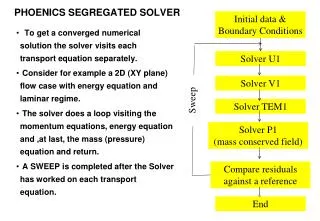
4.6 Solution of Equations •Because the whole equation system is non-linear, the solution procedure is iterative, consisting of the steps of: • computing the imbalances of each of the entities for each cell • computing the coefficients of linear(ised) equations which represent how the imbalances will change as a consequence of (small) changes to the solved-for variables; • solving the linear equations; • correcting the values of solved-for variables, and of auxiliary ones, such as fluid properties, which depend upon them: • repeating the cycle of operations until the changes made to the variables are sufficiently small •Various techniques are used for solving the linear equations: • tri-diagonal matrix algorithm • (a variant of) Stone's 'Strongly Implicit Algorithm', • conjugate-gradient and conjugate-residual solvers
4.7 Boundary Conditions •General form Boundary Conditions are represented in PHOENICS as linearized sources for cells adjacent to boundaries: is termed the COEFFICIENT. is termed the VALUE. is added to , and is added to the RHS of the equation for
4.7 Boundary Conditions •Particular forms For a fixed value boundary, is made very big. The effect is: For a fixed flux boundary, is made very small, and is set to the required flux. Linear and non-linear conditions can be set by appropriate prescription of and
5. Simulation of multi-phase flow in PHOENICS •Multi-phase-flow phenomena are, for PHOENICS, those in which, within the smallest element of space which is considered (the computational cell) several distinguishable materials are present. • Examples: • suspensions of oil droplets in water, or of water droplets in oil; • the air-snow mixture in an avalanche; • the sand-air mixture in a sandstorm; • the "mushy zone" of mixed solid and liquid metal in a casting mould; • the water-air mixture in a shower bath; • the gas-oil-water mixture, in the pores within rock, in a petroleum-recovery process; • droplets of fuel oil mixed with hot gases in a combustion chamber
5. Simulation of multi-phase flow in PHOENICS •Simulation methods in PHOENICS: 1. As two inter-penetrating continua, each having at each point in the space-time domain under consideration, its own: - velocity components, - temperature, - composition, - density, - viscosity, - volume fraction, etc 2. As multiple inter-penetrating continua having the same variety of properties 3. As two non-interpenetrating continua separated by a free surface 4. As a particulate phase for which the particle trajectories are computed as they move through a continuous fluid
1 6. Turbulence models in PHOENICS • The flows which PHOENICS is called upon to simulate are, more often than not, turbulent, by which is meant that they exhibit near-random fluctuations, the time-scale of which is very small compared with the time-scale of the mean-flow, and of which the distance scale is small compared with the dimensions of the domain under study •A broad-brush summary of the satisfactoriness of the most-widely-used turbulence models is: - for predicting time-average hydrodynamic phenomena and the macro-mixing of fluids marked by conserved scalars, the models are "not bad"; but - for the simulation of micro-mixing, which is essential if chemical- reaction rates are to be predicted, they are very poor indeed
2 6. Turbulence models in PHOENICS •Turbulence models in PHOENICS can be classified as belonging to one or other of three groups, namely: • those which employ the Effective Viscosity Hypothesis (EVH) • those which specifically AVOID the EVH • those which may make some INESSENTIAL use of the EVH •Further distinction between models can be made by reference to their handling (or non-handling) of: • heat and mass transfer • chemical reaction • multi-phase effects
3 6. Turbulence models in PHOENICS • Group 1 - which employ the EVH • Sub-group 1.1 in which no differential equations are used • prescribed EV - EV is given a uniform value • LVEL - EV is computed from the velocity, the laminar viscosity and the distance from nearby walls • Prandtl mixing-length - EV is computed from the velocity gradient length and a prescribed length scale • Van-Driest - as for Prandtl mixing length, but with low-Reynolds-number modification • Sub-group 1.2 in which one differential equation is used • Prandtl energy - EV is prescribed-length * SQRT(KE) where KE is energy of turbulence computed from a differential transport equation • Sub-group 1.3 in which 1 or 2 differential equations are used • TWO-LAYER KE-EP - as for KE-EP except that only the KE equation is solved near the wall, where the length scale is treated as known
4 6. Turbulence models in PHOENICS • Sub-group 1.4 in which two differential equations are used • k-epsilon (KE-EP) - EV is proportional to KE**2/EP, where KE and EP (dissipation rate of KE) are computed from differential transport equations • CHEN-KIM KE-EP - as for KE-EP, but with a "dual-time-scale concept" making the formulae depend upon the energy-production rate P • RNG-derived KE-EP - as for KE-EP, but with a "re-normalization- group concept" making the formulae depend upon the energy-production rate P • LAM-BREMHORST - as for KE-EP, but with low-Reynolds number extension requiring knowledge of the distance from the nearest wall • Saffman-Spalding KE-VO - EV is proportional to KE/W**0.5, where KE and W (RMS vorticity fluctuations) are computed from dif. transport eqs. • Kolmogorov-Wilcox KE-OMEGA - EV is proportional to KE/OMEGA, where KE and OMEGA ("turbulence frequency") are from dif. transport eqs. • Sub-group 1.5 in which four differential equations are used • TWO-SCALE KE-EPEV - is computed in a similar manner to that of KE-EP model; but there are two turbulence- energy variables, KP and KT, and two dissipation-rate variables, EP and ET
5 6. Turbulence models in PHOENICS • Group 2 - not employing the EVH • REYNOLDS-stress - EV is not used. Instead, the shear stresses are themselves the dependent variables of differential transport equations, usually six in number • Group 3 - which may or may not employ the EVH • Smagorinsky - EV is used only to resolve the small-scale subgrid-scale motion, the main transfers of momentum being computed by performing three-dimensional time-dependent solutions of the Navier-Stokes equations with the finest affordable space and time sub-divisions • Two-fluid - EV is either not used at all, or is deduced from the local velocity differences between the two intermingling fluids which are used to describe the turbulent fluid mixture • Multi-fluid - as for TWO-FLUID, except that, there being many fluids present, EV can be derived from their various velocities in a wider variety of ways
7. Radiative-heat-transfer models in PHOENICS • A method which is unique to PHOENICS, and is especially convenient when radiating surfaces are so numerous, and variously arranged, that the use of the view-factor-type model is impractically expensive, is IMMERSOL •IMMERSOL method is: • computationally inexpensive; • capable of handling the whole range of conditions from optically-thin (ie transparent) to optically-thick (ie opaque) media; • mathematically exact when the geometry is simple; and • never grossly inaccurate
8. Chemical-reaction processes in PHOENICS • PHOENICS can handle the combustion of gaseous, liquid (e.g. oil-spray) and solid (e.g. pulverized-coal) fuels. • Chemical reactions are simulated by PHOENICS in several ways, including: • SCRS - "the Simple Chemically Reacting System" built into user-accessible Fortran coding • CREK - a set of user-callable subroutines which handle the thermodynamics and finite-rate or equilibrium chemical kinetics of complex chemical reactions • CHEMKIN 2 - the public-domain code to which PHOENICS has an interface • PLANT - which enables users to introduce new reaction schemes and material properties by way of formulae introduced into the data-input command file, Q1
9. Simultaneous solid-stressanalysis • It is frequently required to simulate fluid-flow and heat-transfer processes in and around solids which are, partly as a consequence of the flow, subject to thermal and mechanical stresses • Often it is the stresses which are of major concern, while the fluid and heat flows are of only secondary interest • Engineering examples of fluid/heat/stress interactions: • gas-turbine blades under transient conditions • "residual stresses" resulting from casting or welding • thermal stresses in nuclear reactors during emergency shut-down • manufacture of bricks and ceramics • stresses in the cylinder blocks of diesel engines • the failure of steel-frame buildings during fires
10. Body-fitting in PHOENICS • PHOENICS is enable to compute flows around such bodies by using "body-fitted-coordinate (i.e. BFC) grids"
10. Body-fitting in PHOENICS • PHOENICS possesses its own built-in means of generating such grids; but it can also accept grids created by specialist packages, for example GeoGrid
10. Body-fitting in PHOENICS • PARSOL allows flows around curved bodies to be computed on cartesian grids; and the solutions are often just as accurate as those computed on body-fitted grids.
1 11. PHOENICS Application • Engineering Application: • Aerospace • Automotive • Chemical process • Combustion • Electronics • Marine • Metallurgical • Nuclear • Petroleum • Power • Radiation • Water etc.
2 11. PHOENICS Application • 2. Environment Application: • Atmospheric pollution • Pollution of natural waters • Safety • Fire spread, etc. • 3. Architecture and building science • External flows ( e.g. Flow around bus shelter) • Internal flows (e.g. Ventilation of a Concert Hall) • 4. Other phenomena or features • Physical Models • Chemical Processes • Numerical Methods • Grid Generation, etc.
Chapter 2 The Virtual-Reality Interface