Download
1 / 42
430 likes | 674 Vues
Predicting Weather and Climate with Computers: Numerical Weather Prediction (NWP) Meteo 415 Fall 2012. ENIAC University of Pennsylvania, 1945 ~ 5000 +/- per second. First one-day numerical weather forecast, 1950. NOAA IBM Supercomputer ~4 teraflops/second.

E N D
Predicting Weather and Climate with Computers: Numerical Weather Prediction (NWP) Meteo 415 Fall 2012
ENIAC University of Pennsylvania, 1945 ~ 5000 +/- per second First one-day numerical weather forecast, 1950 • NOAA IBM Supercomputer • ~4 teraflops/second
A round planet in a parallel beam of solar radiation will have strongtemperature gradients from the equator to the poles Temperature gradients create pressure gradients which drive atmospheric motions
Earth system: Atmosphere, hydrosphere, biosphere, cryosphere, geosphere Fluxes of terrestrial energy and mass (water)
Making the Forecast Forecast a quantity F(temp, pressure, humidity, wind) at point x Change in Fbetween now and future time Fat future time + F now = “Initialization”, or “initial conditions” (some from satellite) Need partial differential equation describing rate of change of F
The Equations of Atmospheric Motion Conservation of Momentum Conservation of Energy Conservation of Mass Conservation of Constituent q Equation of State Material Derivative
Constructing an NWP model Grid-point model: Cover 3-D domain with grid of points, solve forecast equations at grid points. Examples: Eta, WRF (Weather Research and Forecast)
Constructing an NWP model Spectral model: atmospheric variables presumed to be wave-like functions (such as sines and cosines). • Spectral models are more attune with wave-like motions in real atmosphere, so they save computational time. • Long-range (beyond 4-day) forecasts usually come from spectral models Examples: GFS (Global Forecast System), European
Atmospheric Numerical Models • Basic Limits • Initial Conditions (resolution) • Boundary Conditions (forces) • Physics (inexact, empirical relationships) • Round-off errors (computational) • Chaos (systemic)
Atmospheric Numerical Models • Starting the Model • Start with first guess field • Usually a 6 hour forecast from same model • Advantages: • On same grid domain with the parameters needed • Reasonable assumption – errors accumulate with time • Computational short-cuts • Adjust with Observations - window of opportunity - discern good v bad reports - automate the process
Satellite Input – Quality Assurance Water Vapor derived winds: 300-700mb [1847 accepted] IR derived winds: 700-1000mb [7048 accepted] IR derived winds: 150-300mb [4653 accepted]
Shortcomings of Model Estimates • Radiative transfer law approximations are applied. • Radiances from several different satellite channels are used together to produce one temperature sounding. • The derived soundings essentially are layer averages in layers defined by the absorber weighting functions for the observed radiation wavelengths. • These are interpolated to much thinner model layers to compare against model fields, or they are interpolated to standard sounding levels and model data are also interpolated to standard sounding levels for comparison.
Shortcomings of Model Estimates • Errors in various packages • Analysis Schemes • Observational (instrument) • Representativeness* • Model physics *Example: Satellite microwave soundings (actually, radiances) over the ocean. These are the only source of temperature profiles in cloudy regions! Resolving only 3 or 4 thick tropospheric levels, they vertically smear out model-resolved tropopause folds and sloping frontal zones. If use of this data degrades the background fields, then the data should be rejected.
Data Reliability • Ascertaining what to keep and throw away
Data Reliability • Ascertaining what to keep and throw away – The No Surprise Snowstorm – Jan 25, 2000
Data Reliability • Known error distributions for GOES in 4DAS
Challenges of Using Satellite Data • Any radiation that's sensed comes from a deep layer of the atmosphere, so vertical resolution is coarser than model vertical resolution • This will improve greatly when interferometers replace radiometers. This is not scheduled on GOES until at least GOES-S • The proper conversion of satellite radiances to temperatures requires knowing the emissivity at the bottom of the layer being sensed. This presents problems over land, so data over land are only reliable for channels sensing the upper troposphere and stratosphere
Atmospheric Numerical Models • The Pitfalls of Data Assimilation SUMMARY • Data Void regions (particularly the oceans) • Bad First Guess Fields • Good Data rejected • Analysis Assumptions
700-mb (~10,000 ft) relative humidity (>70% and >90% shaded green)
Simulating tomorrow’s satellite and radar imagery After-the-fact test case Snowstorm of February 11-13, 2006 (26.9” Central Park) February 11-13, 2006
Simulating tomorrow’s satellite and radar imagery • WRF simulation, • 12 km domain • Clouds are defined using WRF cloud ice (kg/kg) and cloud liquid water (kg/kg)
Comparison of the water vapor image computed using WRF and the radiative transfer model (left) with the observed (by GOES-12) (below)
References The COMET Program: www.meted.ucar.edu/ WeatherVentures, Inc.: www.weatherventures.com/ University of Pennsylvania: www.library.upenn.edu/exhibits/rbm/mauchly/jwm0-1.html
References Fixing Errant Data with Complex Quality Control Collins, W.G., 1997: The use of complex quality control for the detection and correction of rough errors in rawinsonde heights and temperatures: A new algorithm at NCEP/EMC. NCEP Office Note 419, 49 pp. Julian, P.R., 1989: Quality control of the aircraft file at the NMC. Part I. NCEP Office Note 358, 13 pp. [Note - NCEP office notes are scheduled to be available online within a few months of publication of this module] References on Many Aspects of How 3D-VAR Works in the Global Data Assimilation System Derber, J. C., D.F. Parrish, and S. J. Lord, 1991: The new global operational analysis system at the National Meteorological Center. Wea. and Forecasting, 6, 538-547.
References • Derber, J. C. and W.-S. Wu, 1998: The use of TOVS cloud-cleared radiances in the NCEP SSI analysis system. Mon. Wea. Rev., 126, 2287-2299. • McNally, A.P., J.C. Derber, W.-S. Wu, and B.B. Katz, 2000: The use of TOVS level-1B radiances in the NCEP SSI analysis system. Quart. J. Roy. Meteor. Soc., 126, 689-724. • Parrish, D. F. and J. C. Derber, 1992: The National Meteorological Center's spectral statistical interpolation analysis system. Mon. Wea. Rev., 120, 1747-1763. • Spatial Patterns of Model Error Used in 3D-VAR Analysis Derber, J. C. and F. Bouttier, 1999: A reformulation of the background error covariance in the ECMWF global data assimilation system. Tellus, 51A, 195-221