Download
1 / 23
230 likes | 252 Vues
This research discusses the development of a MAPS-based electromagnetic calorimeter for the ILC, providing insights into sensor layout, simulation results, and energy resolution optimization. The innovative design aims for high granularity for improved performance at a reduced cost.

E N D
A MAPS-based digital Electromagnetic Calorimeter for the ILC on behalf of the MAPS group: Y. Mikami, N.K. Watson, O. Miller, V. Rajovic, J.A. Wilson (University of Birmingham) J.A. Ballin, P.D.Dauncey, A.-M. Magnan, M. Noy (Imperial College London) J.P. Crooks, M. Stanitzki, K.D. Stefanov, R. Turchetta, M. Tyndel, E.G. Villani (Rutherford Appleton Laboratory)
Layout Context of this R&D • Introduction to MAPS What is MAPS ? Why for an Electromagnetic CALorimeter ? • The current sensor layout • Sensor simulation • Physics simulation digitisation procedure influence of parameters on theenergy resolution Conclusion LCWS 2007 - Hamburg - A.-M.Magnan (IC London)
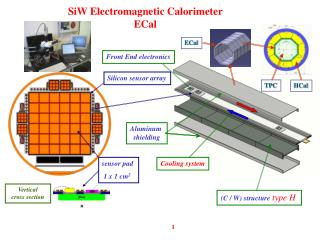
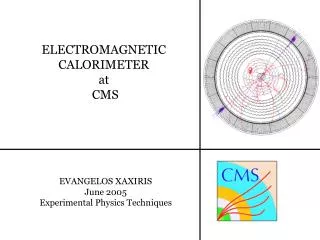
Diode pad calorimeter MAPS calorimeter PCB ~0.8 mm Silicon sensor 0.3mm Tungsten 1.4 mm Embedded VFE ASIC Context of this R&D • Alternative to CALICE Si/W analogue ECAL • No specific detector concept • “Swap-in” solution leaving mechanical design unchanged LCWS 2007 - Hamburg - A.-M.Magnan (IC London)
Introduction to MAPS • MAPS ? MonolithicActivePixelSensor • CMOS technology, in-pixel logic: pixel=sensor+readout electronics • 50x50 μm² : reduces probability of multiple hit per pixel • Collection of charge mainly by diffusion • Why foracalorimeter ? high granularity : better position resolution potentially better PFA performances, or detector more compact reduced cost 1012 pixels : digital readout, DAQ rate dominated by noise Area needed for logic and RAM : ~10% dead area Cost saving : CMOS vs high resistivity Si wafers Power dissipation : more uniform challenge to match analog ECAL 1 μW/mm² LCWS 2007 - Hamburg - A.-M.Magnan (IC London)
Sensor layout : v1.0 submitted ! Design submitted April 23rd, with several architectures. One example: 4 diodes Ø 1.8 um comparator+readout logic analog circuitry. LCWS 2007 - Hamburg - A.-M.Magnan (IC London)
What’s eating charges : the N-well and P-well distribution in the pixels pink = nwell (eating charge) blue = deep p-well added to block the charge absorption INMAPS process • Electronics N-well absorbs a lot of charge : possibility to isolate them ? • INMAPS process : deep P-well implant 1 μm thick everywhere under the electronics N-well. LCWS 2007 - Hamburg - A.-M.Magnan (IC London)
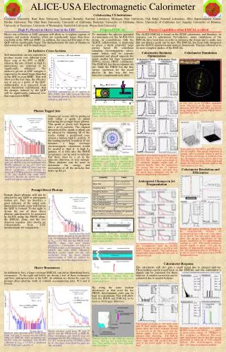
0.9 μm 1.8 μm 3.6 μm The sensor simulation setup Using Centaurus TCAD for sensor simulation + CADENCE GDS file for pixel description • Diode size has been optimised in term of signal over noise ratio, charge collected in the cell in the worse scenario (hit at the corner), and collection time. • Diodes place is restricted by the pixel designs, e.g. to minimise capacitance effects Signal over noise Collected charge LCWS 2007 - Hamburg - A.-M.Magnan (IC London)
50 m 1 21 Cell size: 50 x 50 m2 Whole 3*3 array with neighbouring cells is simulated, and the initial MIP deposit is inputted on 21 points (sufficient to cover the whole pixel by symmetry) Fast simulation for Physics analysis Preliminary results obtained assuming perfect P-well : to reduce the computational time, no N-well or P-well are simulated. Will be compared to a pessimistic scenario with no P-well but a central N-well eating half of the charge. Example of pessimistic scenario of a central N-well eating half of the charge LCWS 2007 - Hamburg - A.-M.Magnan (IC London)
MIP crossing boundaries : effect can be reduced by clustering • So energy resolution is given by the distribution of hits/clusters above threshold: Physics simulation Geant4 energy of simulated hits 0.5 GeV MPV = 3.4 keV σ = 0.8 keV • MAPS Simulation implemented in MOKKA, with LDC01 for now on. • MIP landau MPV stable vs energy @ Geant4 level Assumption of 1 MIP per cell checked up to 200 GeV, • Definition of energy : E α NMIPS. • Binary readout : need to find the optimal threshold, taking into account a 10-6 probability for the noise to fluctuate above threshold. Ehit (keV) 5 GeV MPV = 3.4 keV σ = 0.8 keV Ehit (keV) 200 GeV MPV = 3.4 keV σ = 0.8 keV Ehit (keV) LCWS 2007 - Hamburg - A.-M.Magnan (IC London)
%Einit %Einit %Einit Einit %Einit %Einit %Einit %Einit %Einit Importance of the charge spread : Digitisation procedure Apply charge spread Eafter charge spread Geant4 Einit in 5x5 μm² cells Register the position and the number of hits above threshold + noise only hits : proba 10-6 ~ 106 hits in the whole detector BUT in a 1.5*1.5 cm² tower : ~3 hits. Add noise to signal hits with σ = 100 eV (1 e- ~ 3 eV 30 e- noise) Sum energy in 50x50 μm² cells Esum LCWS 2007 - Hamburg - A.-M.Magnan (IC London)
600 eV thresh Simple clustering A particular event, a particular layer • Loop over hits classified by number of neighbours : • if < 8 : count 1 (or 2 for last 10 layers) and discard neighbours, • if 8 and one of the neighbours has also 8 : count 2 (or 4) and discard neighbours. • Not very optimised : lots of room for improvement ! MeV LCWS 2007 - Hamburg - A.-M.Magnan (IC London)
Neighbouring hit: • hit ? Neighbour’s contribution • no hit ? Creation of hit from charge spread only • All contributions added per pixel • + noise σ = 100 eV • + noise σ = 100 eV, minus dead areas : 5 pixels every 42 pixels in one direction How is the energy affected by each digitisation step ? • E initial : geant4 deposit • What remains in the cell after charge spread assuming perfect P-well LCWS 2007 - Hamburg - A.-M.Magnan (IC London)
MPV-1σ = 2.5 keV • DIGITIZED: • charge spread with perfect P-well assumed, • noise σ=100 eV, • 10-5 probability of a pixel to be above threshold • dead area removed • without or with clustering 16% effect Effect of the clustering on the energy resolution • IDEAL : Geant4 energy, • no charge spread, • no noise, • dead area removed (5 pixels every 42 pixels in one direction) • without or with clustering LCWS 2007 - Hamburg - A.-M.Magnan (IC London)
Effect of charge spread model Optimisticscenario: Perfect P-well after clustering: large minimum plateau large choice for the threshold !! Pessimisticscenario: Central N-well absorbs half of the charge, but minimum is still in the region where noise only hits are negligible + same resolution !!! LCWS 2007 - Hamburg - A.-M.Magnan (IC London)
Effect of dead area and noiseafter clustering Threshold > 600 eV : influence of the noise negligible < 6% effect energy resolution dependant on a lot of parameters : need to measure the noise and the charge spread ! And improve the clustering, especially at high energy. LCWS 2007 - Hamburg - A.-M.Magnan (IC London)
Plans for the summer • Sensor has been submitted to foundry on April 23rd, back in July. • Charge diffusion studies with a powerful laser setup at RAL : • 1064, 532 and 355 nm wavelength, • focusing < 2 μm, • pulse 4ns, 50 Hz repetition rate, • fully automatized • Cosmics and source setup to provide by Birmingham and Imperial respectively. • Work ongoing on the set of PCBs holding, controlling and reading the sensor. • possible beam test at DESY at the end of this year. LCWS 2007 - Hamburg - A.-M.Magnan (IC London)
Conclusion • Sensor v1.0 has been submitted. We aim to have first results in the coming months! • Test are mandatory to measure the sensor charge spread and noise for digitisation simulation. • Once we trust our simulation, detailed physics simulation of benchmark processes and comparison with analog ECAL design will be possible. LCWS 2007 - Hamburg - A.-M.Magnan (IC London)
Thank you for your attention LCWS 2007 - Hamburg - A.-M.Magnan (IC London)
4 diodes Ø 1.8 um same comparator+readout logic Type dependant area: capacitors, and big resistor or monostable Sensor layout : v1.0 submitted ! Design submitted April 23rd : Presampler Preshaper LCWS 2007 - Hamburg - A.-M.Magnan (IC London)
Pre-Shape Pixel Analog Front End Low gain / High Gain Comparator Rst Hit Logic Hit Output Rfb Trim&Mask SRAM SR Cfb Cpre Pre-Sample Pixel Analog Front End Vth+ Vth- Low gain / High Gain Comparator Hit Logic 150ns Rin Cin Preamp Hit Output Shaper Self Reset Trim&Mask SRAM SR PreRst Vrst Cfb Rst Buffer s.f Buffer s.f Cin Preamp 150ns Vth+ Vth- 450ns Reset Sample Cstore THE DesignS big resistor Monostable LCWS 2007 - Hamburg - A.-M.Magnan (IC London)
7 * 6 bits pattern per row 42 pixels 84 pixels Row index The sensor test setup 1*1 cm² in total 2 capacitor arrangements 2 architectures 6 million transistors, 28224 pixels • 5 dead pixels • for logic : • hits buffering (SRAM) • time stamp = BX • (13 bits) • only part with clock lines. Data format 3 + 6 + 13 + 9 = 31 bits per hit LCWS 2007 - Hamburg - A.-M.Magnan (IC London)
Beam background studies purple = innermost endcap radius 500 ns reset time ~ 2‰ inactive pixels • Done using GuineaPig • 2 scenarios studied : • 500 GeV baseline, • 1 TeV high luminosity. LCWS 2007 - Hamburg - A.-M.Magnan (IC London)
Particle Flow: work started ! • Implementing PandoraPFA from Mark Thomson : now running on MAPS simulated files. • First plots with Z->uds @ 91 GeV in ECAL barrel gives a resolution of 35% / √E before digitisation and clustering LCWS 2007 - Hamburg - A.-M.Magnan (IC London)