Download
1 / 44
450 likes | 668 Vues
L. Jay Miller (May 2011) Data Preparation and Gridding for Wind Synthesis Using REORDER, SPRINT, and CEDRIC PROGRAMS. Some Fundamentals of Doppler Radar Velocity Analysis. TRADITIONAL FORMULATION.

E N D
L. Jay Miller (May 2011) Data Preparation and Gridding for Wind Synthesis Using REORDER, SPRINT, and CEDRIC PROGRAMS Some Fundamentals of Doppler Radar Velocity Analysis
TRADITIONAL FORMULATION Radial velocity is projection of particle motion (u,v,w+Vt) onto radar beam (A,E) at several ranges [Vr = (u*sinA + v*cosA)*cosE + W*sinE] Map measurements from (R,A,E) to Cartesian (x,y,z) or coplane (r,s,c) analysis domain Correct each radar for fallspeed contribution Vt = a*(Z^b) * (density correction) Solve 2 or 3 equations Vr = Vr(u,v) or Vr(u,v,w) Include mass continuity equation to obtain the vertical air motion Specify boundary conditions (upper and lower)
Considerations before Gridding • Develop overview of radar scans in context of research goals • Display with SOLOII or CIDD or similar program • Select radar(s) to be used in wind synthesis • Operations in radar sample space before gridding (asymmetries in pulse volume shape) • Preliminary Range-Angle filling and filtering • Correct for fall-speed contribution to Vr • Formats readable by NCAR gridders • REORDER – Universal and Dorade sweep files • SPRINT – Older RP2-7, Universal, Dorade, and NEXRAD Level II (Build 9, MSG1; pre-MSG30)
STEPS 2000 Triple-Doppler Radar NetworkSevereThunderstormElectrification andPrecipitationStudy SPOL KGLD CSU/CHILL
Central Plains Composite 2000.0629.2330 Tornadic (F1) Storm
Considerations for Gridding • Identify characteristics of radar scans • Azimuth-Elevation angle bounds and increments • Range-Height bounds • Determine fields to be interpolated • Radar measured fields (DZ, VE, SW, …) • Ancillary fields (AZ, EL, TIME, …) • Determine latitudes, longitudes of origin and radar(s) to obtain their grid locations • Decide on output grids common to radars
Considerations for Gridding (cont'd) • Issues that control fields to be gridded • Degree of space-time overlap of radar scans • Types and durations of scans (ppi, rhi, …) • Radars (ground-based research, operational, and airborne) • CEDRIC formulation of wind synthesis • Advection needs time field • Airborne needs azimuth and elevation angles • Gridder to be used (SPRINT or REORDER)
Local ENU-ECEF *Convert radar lat-lon-height to Cartesian coordinates of common output grid ENU – local tangent plane ECEF – Center of the Earth • X along prime meridian (0 deg reference dividing East and West longitudes at the equator) • Z points to North Pole • Lambda – longitude of local point • Phi – latitude of local point • Spherical Earth with 4/3 radius
REORDER ALGORITHM Region of influence (box) Cartesian (xyz radii or box half-dimensions) Spherical (rae radii dependent on slant range) Hybrid (Cartesian until exceeded by Spherical) Filter or distance-weighting scheme applied to all measured values inside the box Cressman (Rsq – rsq)/(Rsq + rsq) Exponential [exp(-a*rsq/Rsq) Big Rsq – sum of box radii squared Little rsq – squared distance (RAE sample – XYZ grid) Uniform weighting and closest point
REORDER RADII of INFLUENCE Cartesian radii: (xradius, yradius, zradius) If xradius = 0, then xradius = yradius Map into cartesian (dx, dy, dz) box Spherical radii: (rgradius, azradius, elradius) Always map into cartesian (dx, dy, dz) box User inputs (azradius, elradius) in degrees dy (dz) = range*[azradius (elradius) in radians] If rgradius = 0, dx = range*(azradius in radians) If rgradius > 0, then dx = constant rgradius km Hybrid radii: Uses cartesian radii until spherical radii are bigger, then shifts to spherical
ORIENTATION of GRIDDING BOXES REORDER* Prefer SPRINT-LIKE *Inner (outer) box – Fixed (range-dependent) size
KGLD – REORDER (part 1) DATA LOCATION & RADAR LAT/LON/ALT Grid (G) Radar (R) XYZ Grid
KGLD – REORDER (part 2) WEIGHTS BOX Dimensions XYZ Radii RAE Radii
KGLD – REORDER (part 3) Fields to be Interpolated Data Quality Study Volume Time Interval
SPRINT ALGORITHM Successive linear interpolations in the R, A, E directions Uses 8 RAE sample gates surrounding the output grid point Two ranges Two azimuths Two elevations XYZ, XYE, XYC, LLZ, or LLE
KGLD – SPRINT Input (part 1) INPUT DATA LAT/LON/ALT 2D FILTER Range-Angle
KGLD – Sprint Input (part 2) DZ Pass VE Pass VE Pass DATE-TIME
Regions Influencing Output Fields XY output grid (Big +s) RA sampling locations (Little +s) REORDER circles for Cartesian radii SPRINT RA Cells
LOCAL UNFOLDING & QUAL NOTE: Currently Reorder and Sprint use standard deviation rather than velocity variance and output 100*Q. M below is the number of range gates in a range slab (for Sprint M = 2). QUAL includes only those velocities used for individual output grid point. Va = 2*Vn Ue = Local estimate at output XYZ NOTE
COordinated coPLANar Scanning Modify elevation angle: tan (E) = tan (coplan angle) * abs [sin (A -Ab)]
COPLAN Interpolation with SPRINT and Winds with CEDRIC Two-dimensional Winds: Orthogonalize V1 and V2 into Ur and Us
SPOL – REORDER Scan Information Elevation Angles Azimuthal Spacing
CSU/CHILL – REORDER Scan Info Elevation Angles Azimuthal Spacing
KGLD – REORDER Scan Information Elevation Angles Azimuthal Spacing
SPOL - PPI (RAE) vs CEDRIC (XYE) DZ @ E=0.5 deg XYE - Threshold at LDR < -6 VE @ E=0.5 deg Both – Threshold at LDR < -6
SPOL -Sprint vs Reorder (DZ) Z = 2.5 km MSL UL = SPRINT UR = REORDER CRE-XYZ radii 0.5-0.5-1.0 km LL = REORDER EXP-RAE radii 0.2-1.0-1.0 km-dg LR = REORDER CRE-RAE radii 0.0-1.0-1.0 deg
SPOL – Sprint vs Reorder (DZ) Z = 7.5 km MSL UL = SPRINT UR = REORDER CRE-XYZ radii 0.5-0.5-1.0 km LL = REORDER EXP-RAE radii 0.2-1.0-1.0 km-dg LR = REORDER CRE-RAE radii 0.0-1.0-1.0 deg
SPOL – Sprint vs Reorder (DZ) Z = 13.5 km MSL UL = SPRINT UR = REORDER CRE-XYZ radii 0.5-0.5-1.0 km LL = REORDER EXP-RAE radii 0.2-1.0-1.0 km-dg LR = REORDER CRE-RAE radii 0.0-1.0-1.0 deg
Global Unfolding with CEDRICTemplate creation and cleanup Preliminary unfold with vertical profile of VE Additional steps to further unfold AUTO – Decimate, global fill, and unfold AUTOTEMP – Propagate away from LEVEL AUTOFILL – Like AUTOTEMP, propagate and fill Unfold VE → VEUF using the above template Decimate, filter, and fill with multiple PATCHER
SPOL – Sprint vs Reorder (VE) Z = 2.5 km MSL UL = SPRINT UR = REORDER CRE-XYZ radii 0.5-0.5-1.0 km LL = REORDER EXP-RAE radii 0.2-1.0-1.0 km-dg LR = REORDER CRE-RAE radii 0.0-1.0-1.0 deg
SPOL – Sprint vs Reorder (VEUF) Z = 2.5 km MSL UL = SPRINT UR = REORDER CRE-XYZ radii 0.5-0.5-1.0 km LL = REORDER EXP-RAE radii 0.2-1.0-1.0 km-dg LR = REORDER CRE-RAE radii 0.0-1.0-1.0 deg
SPOL – Sprint vs Reorder (VE) Z = 7.5 km MSL UL = SPRINT UR = REORDER CRE-XYZ radii 0.5-0.5-1.0 km LL = REORDER EXP-RAE radii 0.2-1.0-1.0 km-dg LR = REORDER CRE-RAE radii 0.0-1.0-1.0 deg
SPOL-Sprint vs Reorder (VEUF) Z = 7.5 km MSL UL = SPRINT UR = REORDER CRE-XYZ radii 0.5-0.5-1.0 km LL = REORDER EXP-RAE radii 0.2-1.0-1.0 km-dg LR = REORDER CRE-RAE radii 0.0-1.0-1.0 deg
SPOL – Sprint vs Reorder (VE) Z = 13.5 km UL = SPRINT UR = REORDER CRE-XYZ radii 0.5-0.5-1.0 km LL = REORDER EXP-RAE radii 0.2-1.0-1.0 km-dg LR = REORDER CRE-RAE radii 0.0-1.0-1.0 deg
SPOL – Sprint vs Reorder (VEUF) Z = 13.5 km MSL UL = SPRINT UR = REORDER CRE-XYZ radii 0.5-0.5-1.0 km LL = REORDER EXP-RAE radii 0.2-1.0-1.0 km-dg LR = REORDER CRE-RAE radii 0.0-1.0-1.0 deg
Horizontal-Vertical Resolutionfrom Range-Elevation Angle Resolution Z = R*sinE dZ = dR*sinE + RdE*cosE H = R*cosE dH = dR*cosE - RdE*sinE dZ ~ RdE @ 0 to dR @ 90 dH ~ dR @ 0 to RdE @ 90
Summary Comparison of Reorder and Sprint REORDERSPRINT SCHEME: DISTANCE-WEIGHTING TRI-LINEAR INTERPOLATION CLOSEST POINT CLOSEST POINT UNIFORM-WEIGHTING REGION OF INFLUENCE: USER-SPECIFIED RADII LOCALLY ADAPTIVE XYZ-ORIENTED RAE-ORIENTED CONSEQUENCES: CONSTANT LINEAR SCALE UNEQUAL LINEAR SCALE UNEQUAL ERROR CONSTANT ERROR GROUND-BASED (AIRBORNE) OUTPUT GRID ORIENTATION: USER SPECIFIES + X AZIMUTH USER SPECIFIES + X AZIMUTH (USER-SPECIFIES + X AZIMUTH) (+ X – OUT RIGHT SIDE) (+ Y – FLIGHT DIRECTION) (ROTATE TO SPECIFIED + X AZIMUTH)