Morphological Operators
Morphological Operators. More on Homogeneous Intensity Regions. Morphology Refers to “form and structure” Defined as set operations Pixels that make up a region are the elements of the set Pixels not in the region are the elements outside the set


Morphological Operators
E N D
Presentation Transcript
More on Homogeneous Intensity Regions • Morphology • Refers to “form and structure” • Defined as set operations • Pixels that make up a region are the elements of the set • Pixels not in the region are the elements outside the set • Operate on binary images where connected components have been identified • Basic implementation is similar to that of convolution with a kernel
Pixels as Sets 1 3 2 5 4 1 Set of pixels (white) 5 Sets of pixels (connected components with boundaries)
Morphology Operations • Inputs • Binary image (connected components) • Structuring element (kernel) • Output • Processed regions Region Region Morphological Operation Structuring Element
Structuring Element • Analogous to a convolution kernel • Acts as a “probe” of the binary image • Designate an origin of the element • May be the central pixel • May be some other pixel • Can be any shape or size
Structuring Element • Notice the empty spaces on the elements • These spaces are treated as “don’t cares” • Clearly we must represent them as something when writing code • You choose what the values should be and make sure you handle them consistently • More on this later
Basic Operations • Five common Morphological Operations • Dilation • Erosion • Closing • Opening • Hit And Miss
Dilation • Used to enlarge a region • Sweep the structuring element over the image (as you did with convolution) • Each time the origin lands on a pixel within the region… • Write a 1 wherever the structuring element is a 1 • That is, replicate the structuring element for every region pixel • The effect will be to thicken lines, fill gaps and holes, and grow object boundaries
Dilation With a 3x3 structure element of all 1’s: INPUT OUTPUT DIFFERENCE
Erosion • Used to shrink a region • Sweep the structuring element over the image • When all structuring elements (the 1’s) cover region pixels • Place a 1 at the origin pixel of the output image • The effect will be to thin lines and shrink object boundaries
Erosion With a 3x3 structure element of all 1’s: INPUT OUTPUT DIFFERENCE
Closing • Used to close internal holes and eliminate concavities from regions • Concatenation of dilation/erosion operations • Perform a dilation on the input image to produce an intermediate image • Perform an erosion on the intermediate image to produce the output image
Closing With a 3x3 structure element of all 1’s: INPUT OUTPUT DIFFERENCE
Opening • Used to remove “tails” from regions • Concatenation of erosion/dilation operations • Perform an erosion on the input image to produce an intermediate image • Perform an dilation on the intermediate image to produce the output image
Opening With a 3x3 structure element of all 1’s: INPUT OUTPUT DIFFERENCE
INPUT DILATE ERODE OPEN CLOSE Another Example With a 3x3 structure element of all 1’s:
Hit And Miss • Searches for specific patterns in the image • Sweep the structuring element over the image • When all structuring elements match underlying image pixels exactly • Consider structure element 1’s (region pixels), 0’s (non-region pixels), and “don’t cares” • Logical OR the image pixel corresponding to the structure element origin into the output image (i.e. write a value to the output where the origin of the structuring element is)
Hit And Miss • Note that the Structuring Element contains three types of values • Foreground (region) indicators • Background (non-region) indicators • “don’t care” indicators • Foreground indicators must land on region pixels • Background indicators must land on non-region pixels • Don’t care indicators can land on anything
Hit And Miss STRUCTURING ELEMENT OUTPUT INPUT There is a white pixel here (lower left corner of the square)
Compound Operations • Advanced operations can be created by combining the basic operations • Skeletonization (thinning) • Thin(i, j) = I(i, j) ∩ HitAndMiss(I(i, j)) • This will take a “wide” object and produce a thin object
From Edges to Lines The Hough Transform
From Edges To Lines • Edges are a good start • They contain some important information and reduce the amount of raw data • We don’t have to deal with all the pixel intensities that may not be all that informative • But now we must do something with the edges • As we saw last week, computing texture was one of the things we can do
Hough Transform Hough Transform Binarized edgels (edge pixels), not a line!
Hough Transform Hough Transform Binarized edgels (edge pixels), not a line!
Hough Transform Hough Transform Binarized edgels (edge pixels), not a line!
Hough Transform Hough Transform Binarized edgels (edge pixels), not a line!
Hough Transform Hough Transform Binarized edgels (edge pixels), not a line!
Hough Transform Hough Transform Binarized edgels (edge pixels), not a line!
Hough Transform Hough Transform Binarized edgels (edge pixels), not a line!
Hough Transform Hough Transform Binarized edgels (edge pixels), not a line!
Hough Transform • What exactly is going on? • The Hough Transform is a technique for finding straight lines in a mass of disconnected points • It’s a “model-based” technique • It utilizes a mathematical equation (a model) of a line and then tries to fit points to the equation
Hough Transform • Input image is [typically] a binarized edge magnitude map • You could define it to use edge magnitudes in a manner similar to the Canny edge detector • The process maps image space edge points to Hough Space coordinates • The output image is the location of lines in image space • What I showed was a rendering of Hough space which is not really the desired output
Hough Space • A line in image space maps to a point in Hough Space • A point in image space maps to multiple points in Hough Space • Each point (ρ, θ) in Hough space represents line in image space • ρ is the perpendicular distance from the line to the origin • θ is the orientation of the line relative to a specified axis
Hough Transform • A single edge point in image space can be part of an infinite number of lines in image space • Since “infinite” is a bit difficult to deal with in the digital computer world we quantize the orientation of the lines into convenient bins • To compute the Hough Transform of a single point in image space we measure the distance from the origin to every possible line through the point
ρ ρ θ θ Hough Transform • Specifically, we compute for all values of θ. For example: Xp, Yp Xp, Yp
Hough Space • The result is a sinusoidal waveform in Hough space There is a single dot in here
ρ θ Implementation • Basic data structure is the accumulator matrix • Similar to intensity histogram creation • Initialize each location to 0 • Set θ • Calculate ρ • Increment the (ρ, θ) bin
Mechanization • When multiple dots contribute to the same line (are colinear) in image space the sin waves will intersect in a single point in Hough Space • The coordinates of that point represent the parameters of the line
Implementation Considerations • Must settle on an origin • Upper left image corner • Image center • Lower left image corner • Whatever • Just choose one and document it • Must select a quantization of the orientation • Too fine of a quantization and the sinusoidal waves won’t intersect in a single point • Too coarse of a quantization and near parallel lines are accumulated into a single bin
Implementation Considerations • The image points won’t always be perfectly collinear and therefore the Hough Space sinusoidal waves won’t always intersect in a single point • Angle quantization • Non-maximal peak suppression on the Hough accumulator array may be employed to reduce clustering effects (similar to the process used by Canny)
Implementation Considerations The answer is in here somewhere
Implementation Considerations • After non-maximal peak suppression you may want to binarize (threshold) the accumulator array leaving only the strongest peaks • Those represent locations where the most sinusoids intersected • This is where the most number of points contributed to a given line (high degree of colinearity)
Implementation Considerations • The basic Hough Transform does not keep track of which points contribute to a line • Make each accumulator bin a linked-list (or array) of image space point locations if you want to do this • Edge orientation information is completely ignored • May want to store this or use it to weight a particular edges contribution to the accumulator
“Gotchas” • Make sure your accumulator array is initialized to 0 each time you compute a Hough Transform • Make sure your accumulator array is big enough to hold all possible distances • Distances can be as far as the diagonal length of the image • Distances can be positive or negative dependent on how you choose your origin
Generalized Hough Transform • The only thing specific to a straight line is the parameterization – the process is general • Basically, any shape that can be quantitatively described can be detected with the Hough Transform • Many approaches to detecting circles have been published – especially fixed radius circles