Seminar Lectures in Remote Sensing of Earth-Atmosphere: Spectral Characteristics and Energy Sources
520 likes | 570 Vues
Explore the spectral characteristics of energy sources in satellite remote sensing, focusing on solar and Earth-emitted energy. Understand how the atmosphere and Earth's surface interact with incoming radiation and reflections. Learn about radiative transfer through the atmosphere and spectral bands used in sensing systems. Gain insights into detecting barren regions and inferring surface properties based on high spectral resolution data.

Seminar Lectures in Remote Sensing of Earth-Atmosphere: Spectral Characteristics and Energy Sources
E N D
Presentation Transcript
SummaryRemote Sensing SeminarLectures in BertinoroPaul MenzelNOAA/NESDIS/ORA23 Aug – 2 Sep 2004
Satellite remote sensing of the Earth-atmosphere Observations depend on telescope characteristics (resolving power, diffraction) detector characteristics (signal to noise) communications bandwidth (bit depth) spectral intervals (window, absorption band) time of day (daylight visible) atmospheric state (T, Q, clouds) earth surface (Ts, vegetation cover)
Spectral Characteristics of Energy Sources and Sensing Systems
Solar (visible) and Earth emitted (infrared) energy Incoming solar radiation (mostly visible) drives the earth-atmosphere (which emits infrared). Over the annual cycle, the incoming solar energy that makes it to the earth surface (about 50 %) is balanced by the outgoing thermal infrared energy emitted through the atmosphere. The atmosphere transmits, absorbs (by H2O, O2, O3, dust) reflects (by clouds), and scatters (by aerosols) incoming visible; the earth surface absorbs and reflects the transmitted visible. Atmospheric H2O, CO2, and O3 selectively transmit or absorb the outgoing infrared radiation. The outgoing microwave is primarily affected by H2O and O2.
VIIRS, MODIS, FY-1C, AVHRR CO2 O2 H2O O2 H2O H2O H2O O2 H2O H2O CO2
AVIRIS Movie #2 AVIRIS Image - Porto Nacional, Brazil 20-Aug-1995 224 Spectral Bands: 0.4 - 2.5 mm Pixel: 20mx 20mScene: 10km x 10km
MODIS MODIS IR Spectral Bands
GOES-12 Sounder – Radiances – all bands from 14.7 to 3.7 um and vis
line broadening with pressure helps to explain weighting functions ABC High Mid Low A B C ABC
AIRS Spectra from around the Globe 20-July-2002 Ascending LW_Window
Sensitivity of High Spectral Resolution to Boundary Layer Inversions and Surface/atmospheric Temperature differences (from IMG Data, October, December 1996)
Twisted Ribbon formed by CO2 spectrum: Tropopause inversion causes On-line & off-line patterns to cross 15 m CO2 Spectrum Blue between-line Tbwarmer for tropospheric channels,colder for stratospheric channels --tropopause-- Signature not available at low resolution
Silicate (ash cloud) signal at Anatahan, Mariana Is Image is ECMWF bias difference of 1227 cm-1 – 984 cm-1 (double difference) obs obs - clear sky calc Note slope
Note slope Cirrus signal at Anatahan Image is ECMWF Tb bias difference of 1227 cm-1 – 781 cm-1 (double difference) obs obs - clear sky calc
Inferring surface properties with AIRS high spectral resolution data Barren region detection if T1086 < T981 T(981 cm-1)-T(1086 cm-1) Barrenvs Water/Vegetated T(1086 cm-1) AIRS data from 14 June 2002
Aerosol Size Distribution • There are 3 modes : • - « nucleation »: radius is between 0.002 and 0.05 mm. They result from combustion processes, photo-chemical reactions, etc. • - « accumulation »: radius is between 0.05 mmand 0.5 mm. Coagulation processes. • - « coarse »: larger than 1 mm. From mechanical processes like aeolian erosion. • « fine » particles (nucleation and accumulation) result from anthropogenic activities, coarse particles come from natural processes. 0.01 0.1 1.0 10.0
Radiance data in 6 bands (550-2130nm). • Spectral radiances (LUT) to derive the aerosol size distribution • Two modes (accumulation 0.10-0.25µm; coarse1.0-2.5µm); ratio is a free parameter • Radiance at 865µm to derive t Aerosols over Ocean Normalized to t=0.2 at 865µm • Ocean products : • • The total Spectral Optical thickness • • The effective radius • • The optical thickness of small & large modes/ratio between the 2 modes
MODIS TPW Clear sky layers of temperature and moisture on 2 June 2001
Definitions of Radiation __________________________________________________________________ QUANTITY SYMBOL UNITS __________________________________________________________________ Energy dQ Joules Flux dQ/dt Joules/sec = Watts Irradiance dQ/dt/dA Watts/meter2 Monochromatic dQ/dt/dA/d W/m2/micron Irradiance or dQ/dt/dA/d W/m2/cm-1 Radiance dQ/dt/dA/d/d W/m2/micron/ster or dQ/dt/dA/d/d W/m2/cm-1/ster __________________________________________________________________
Using wavenumbers c2/T Planck’s Law B(,T) = c13 / [e -1] (mW/m2/ster/cm-1) where = # wavelengths in one centimeter (cm-1) T = temperature of emitting surface (deg K) c1 = 1.191044 x 10⁻⁵ (mW/m2/ster/cm-4) c2 = 1.438769 (cm deg K) Wien's Law dB(max,T) / dT = 0 where (max) = 1.95T indicates peak of Planck function curve shifts to shorter wavelengths (greater wavenumbers) with temperature increase. Stefan-Boltzmann Law E = B(,T) d = T4, where = 5.67 x 10⁻⁸ W/m2/deg4. o states that irradiance of a black body (area under Planck curve) is proportional to T4 . Brightness Temperature c13 T = c2/[ln(______ + 1)] is determined by inverting Planck function B
A1 1 = A2 / R2 R A2 Telescope Radiative Power Captureproportional to throughput A Spectral Power radiated from A2 to A1 = L() A11mW/cm-1 Instrument Collection area Radiance from surface = L()mW/m2 sr cm-1 Earth pixel {Note: A1 A2 / R2= A11= A22 }
Radiative Transfer Equation When reflection from the earth surface is also considered, the RTE for infrared radiation can be written o I = sfc B(Ts) (ps) + B(T(p)) F(p) [d(p)/ dp] dp ps where F(p) = { 1 + (1 - ) [(ps) / (p)]2 } The first term is the spectral radiance emitted by the surface and attenuated by the atmosphere, often called the boundary term and the second term is the spectral radiance emitted to space by the atmosphere directly or by reflection from the earth surface. The atmospheric contribution is the weighted sum of the Planck radiance contribution from each layer, where the weighting function is [ d(p) / dp ]. This weighting function is an indication of where in the atmosphere the majority of the radiation for a given spectral band comes from.
RTE in Cloudy Conditions Iλ = η Icd + (1 - η) Ic where cd = cloud, c = clear, η = cloud fraction λ λ o Ic = Bλ(Ts) λ(ps) + Bλ(T(p)) dλ . λ ps pc Icd = (1-ελ) Bλ(Ts) λ(ps) + (1-ελ) Bλ(T(p)) dλ λ ps o + ελ Bλ(T(pc)) λ(pc) + Bλ(T(p)) dλ pc ελ is emittance of cloud. First two terms are from below cloud, third term is cloud contribution, and fourth term is from above cloud. After rearranging pc dBλ Iλ - Iλc = ηελ(p) dp . ps dp Techniques for dealing with clouds fall into three categories: (a) searching for cloudless fields of view, (b) specifying cloud top pressure and sounding down to cloud level as in the cloudless case, and (c) employing adjacent fields of view to determine clear sky signal from partly cloudy observations.
Cloud Properties RTE for cloudy conditions indicates dependence of cloud forcing (observed minus clear sky radiance) on cloud amount () and cloud top pressure (pc) pc (I - Iclr) = dB . ps Higher colder cloud or greater cloud amount produces greater cloud forcing; dense low cloud can be confused for high thin cloud. Two unknowns require two equations. pc can be inferred from radiance measurements in two spectral bands where cloud emissivity is the same. is derived from the infrared window, once pc is known. This is the essence of the CO2 slicing technique.
Cloud Clearing For a single layer of clouds, radiances in one spectral band vary linearly with those of another as cloud amount varies from one field of view (fov) to another Clear radiances can be inferred by extrapolating to cloud free conditions. clear RCO2 x partly cloudy xx x x x x cloudy x x N=1 N=0 RIRW
Moisture Moisture attenuation in atmospheric windows varies linearly with optical depth. - ku = e = 1 - k u For same atmosphere, deviation of brightness temperature from surface temperature is a linear function of absorbing power. Thus moisture corrected SST can inferred by using split window measurements and extrapolating to zero k Moisture content of atmosphere inferred from slope of linear relation.