Download
1 / 34
340 likes | 348 Vues
Canadian Activities with Regard to TEMPO. Chris McLinden and Richard M é nard Environment Canada 24 July 2013. Outline. Canadian Interest in TEMPO Current activities and links to TEMPO Air Quality Forecast Program Chemical Forecast Models (Regional and High Resolution)

E N D
Canadian Activities with Regard to TEMPO Chris McLinden and Richard Ménard Environment Canada 24 July 2013
Outline • Canadian Interest in TEMPO • Current activities and links to TEMPO • Air Quality Forecast Program • Chemical Forecast Models (Regional and High Resolution) • Chemical Data Assimilation • Capacity to perform OSSE’s • Model Validation with Satellites • Satellite Derived Emissions • Oil Sands Monitoring • Challenges (Algorithm, Resolution, …) • Canadian Contribution to TEMPO
Canadian Interest in TEMPO (1/2) • Environment Canada Air Quality Forecast Program. Monitoring and real time objective analysis of surface NO2 and PM for the Air Quality Health Index (AQHI) program • Monitoring of large sources of pollutants: urban areas, industrial locations (e.g., oil sands, smelters, ...) • Transboundary pollution transport monitoring • Quantification of emissions – individual sources, source regions • Monitoring of wildfire, volcanic plumes, and other sporadic emission events • Detection and tracking of emerging hot spots; e.g., rapid expansion of liquefied natural gas production (hydraulic fracking) in northern British Columbia
Canadian Interest in TEMPO (2/2) • Deposition of NO2, SO2 (e.g., acid sensitive lakes in N. Saskatchewan) Surface concentrations are also of interest for epidemiological exposure studies • Chemical data assimilation – operational AQ forecasts • Algorithm development for aspects of particular relevance for Canada: • Stratospheric NO2 removal; e.g., assimilation of stratospheric NO2 profiles from other (proposed) missions • Belgian Altius mission • Canadian CASS (ACE-FTS2, OSIRIS2) mission • Retrievals over snow • High viewing angles
Canadian Air Quality Forecast Program • Ten year old program that has evolved from an O3-only forecast in Eastern Canada to a Canada-wide O3, NO2, PM2.5 forecast program • Forecast is communicated in most areas as an Air Quality Health Index (AQHI) AQHI = 10/10.4100[(exp(0.000871[NO2])-1) +(exp(0.000537[O3]) -1)+(exp(0.000487[PM2.5]) -1)] • 10 point scale that links air quality to the health risk associated with exposure to a 3 pollutant mixture • Developed by Health Canada (Stieb et al., 2008, JA&WMA ) from Canadian multi-city mortality/morbidity studies of short term health effects and AQ data from the Canadian National Air Pollution Surveillance Network (NAPS)
TEMPO Relevance for Canada From Kelly Chance, SAO • TEMPO coverage of Canada: • ~99.5% of Canadian population • >50% of territory • Sparsely populated, often no monitoring stations nearby • Stats Canada 2008 cause-of-death statistics: Total deaths 238,617 Crime 565 Skin Cancer 901 Respiratory Diseases 20,728 ~21,000 Canadian deaths due to air pollution in 2008. The majority of these will be from the chronic effects of long term exposure, but over 2,600 will be from acute short term recent exposure The economic costs of treatment of air pollution effects will top C$8 billion in 2008, accumulating to over C$250 billion by 2030. Respiratory Diseases 20,728 Respiratory Diseases 20,728 National Post, November 2011
Canadian Air Quality Forecast Suite: Operational Model PM2.5 NO2 Ozone • 3D, continental-wide, hourly forecasts of PM2.5, O3 and NO2, twice a day (00 and 12 UTC), for the next 48h • Publicly accessible at http://www.weatheroffice.gc.ca (Analyses& Modelling) • Forecasts are based on GEM-MACH: multi-scale chemical weather forecast model composed of dynamics, physics, and in-line chemistry modules • Weather forecast suite not merged with air quality forecast suite: • AQ runs launched after completion of weather forecast with repeat of meteorology
Canadian AQ Forecast Suite : Operational Configuration:GEM-MACH10 • GEM-MACH options chosen to meet EC’s operational AQ forecast needs; key characteristics include: • limited-area (LAM) configuration where grid points are co-located with operational met-only GEM which supplies initial conditions and lateral boundary conditions for GEM-MACH10 • 10-km horizontal grid spacing, 80 vertical levels to 0.1 hPa • 2-bin sectional representation of PM size distribution (i.e., 0-2.5 and 2.5-10 μm) with 9 chemical components • Some processes resolved with increased number of bins operational Oct 2012 GEM-10 grid (blue) ; GEM-MACH10 grid (red) • Full process representation of oxidant and aerosol chemistry: • gas-, aqueous- & heterogeneous chemistry mechanisms • aerosol dynamics • dry and wet deposition (including in and below cloud scavenging)
Summer 2012 Average Forecasts surfaceO3 (ppb) surface NO2 (ppb) surface PM2.5 (g/m3)
High Resolution (2.5 km) Modelling Support for Satellite Studies at EC • Example: • Comprehensive on-line air-quality model forecasts at 2.5km resolution for Alta./Sask. • These forecasts include total column and emissions into the column of several gases, for comparison to satellite observations. • Below: Column NO2 forecast for 20UT, July 17, 2013. Entire model domain. Zoom-in on Oil Sands Courtesy of Paul Makar (Environment Canada)
fine particles ozone Operational objective analysis Regional 10 km – O3, PM2.5, (NO2, SO2, CO) each hour experimental since 2003, operational Feb 2013 soon available on Weather Office http://weather.gc.ca/mainmenu/airquality_menu_e.html
OA average summer 2012 OA Real-time, hourly averaged analysis increments zoom in OA near Toronto Objective analysis of NO2
Stratospheric chemical data assimilationexperimental since 2005 – collaboration with BiRA Mesospheric descent: With assimilation, proper error stats, analyses do take this NO2 into account even though the model does not (Robichaud et al. 2010, ACP) • Free model run: good agreement with FTIR O3, HCl, ClONO2, HNO3 • Not so good with NO2 (tropics, upper strat, mesospheric descent) • but assimilation makes a significant difference
Chemical DA : plans • EC Meteo has an operational 4D-Var and EnKF and they are moving towards an EnVar next year • GEM-MACH, GEM-BACH coupled meteo-chem 3DVar • Stratospheric BASCOE CTM, 4D-Var (Quentin and Menard 2012) & EnKF (Skachko et al 2013, submitted) and moving towards hybrid EnVar with parameter estimation next year (collaboration with BIRA) • Plan at EC for the next 5 years. EnVar of AQ GEM-MACH
Sample OSSE Results – Environment Canada Ozone Analyses Mean Errors (Relative to Nature Run) for January 2006 South pole (-90 to -60) S. mid-latitude (-60 to -30) Tropics (-30 to 30) Control (SBUV/2) MLS (+SBUV/2) IRLS (+SBUV/2) N. mid-latitude (30 to 60) North pole (60 to 90) Global Courtesy of Yves Rochon et al. (Environment Canada)
Model Validation Using Satellites • OMI – GEM-MACH comparisons, mean NO2 tropospheric VCD (Nov 2010 – Oct 2011) OMI GEM-MACH, sampled as OMI Courtesy of Cristen Adams (Environment Canada)
OMI (2005-2011 average) Oil Sands Monitoring NO2: DOMINO v2 NO2: DOMINO v2 EC AMFs NO2: SPv2.1 EC AMFs NO2: SP v2.1 SO2: NASA PBL EC AMFs SO2: NASA PBL
Satellite-Derived Emissions • Emissions derived from OMI, SCIAMACHY, and GOME2 • SCIAMACHY and GOME2 detection limit ~300 t[SO2]/yr • about 30 isolated sources can be detected adapted from Fioletov et al., JGR, in press
OMI SO2 “catalogue” • OMI detection limit ~70 t[SO2]/yr; >200 sources can be detected • emissions derived by tracking downwind decay of SO2 Industrial courtesy of Vitali Fioletov, EC
Algorithm Challenges • Snow detection • Changing reflectivity • Aerosols, cloud fraction, ... 2000-2001 2002-2004 2011-2012 2005-2007 2008-2010 Reflectivity MODIS reflectivity, summer average
Canadian Contribution to TEMPO (1/2) • Very high interest in TEMPO by Environment Canada for the AQ forecasting program • Interest expected from Other Canadian Government Departments: • Health Canada • Natural Resources Canada / Canadian Forestry Services • Agriculture and Agri-Foods Canada –AAFC • Canadian Universities interested (e.g. Dalhousie U. and others TBD) • Canadian Space Agency looking into the co-funding of Canadian TEMPO R&D activities • EC planning to host TEMPO workshop in November 2013
Canadian Contribution to TEMPO (2/2) • TEMPO-directed R&D (EC, OGD, Universities) • Organized under a Canadian-TEMPO science team • Co-funded by CSA • Development of work plan • TEMPO validation over Canada (<60ºN) • GB remote sensing (6 Brewer stations, 14 Aeronet, FTIRs, aerosol lidars) • Ozonesonde stations (7) • Surface monitoring stations (~140) • Pandoras • Validation campaigns • TEMPO Stratospheric NO2 CDA • Altius (Belgium project – Phase B) • CASS (CSA project)
First EC Pandora results - ozone • Pandora placeholder Pandora 103 & 104 operating at EC HQ (Toronto) 104 scheduled for deployment at oil sands + Pandora 104 (increased by 4.5%) Brewer 145
ALTIUS is a limb sounder spectrometer, capable of a 0.5 km vertical sampling. It consists of three independent spectral camera’s (optics+AOTF+2-D imager) in the UV-Vis-NIR range (250-1800 nm). (P.I. Dider Fussen, BIRA) The instrument, on board a heliosynchronous micro-satellite, is operated in a multi-mode approach (limb, solar occ, stellar occ) using nominal and campaign/calibration scenarios. It allows for 3-D atmospheric tomography. The main geophysical targets are strato/mesospheric ozone profiles and minor trace gases (NO2,H2O, BrO, CH4, aerosols, temperature..).
EC reprocessing of OMI data over oil sands NO2: Level 1, calibrated spectra Step in retrieval Use existing KNMI retrieval, redo 3rd step 1 Spectral analysis NASA KNMI Removal of stratosphere: high pass filtering Removal of stratosphere: modelling stratospheric NO2 2 EC Calculation of Air Mass Factors Calculation of Air Mass Factors Calculation of Air Mass Factors 3 Level 2, tropospheric VCD Level 2, tropospheric VCD Level 2, tropospheric VCD
Application to oil sands monitoring • Surface mining & upgrading processes emit NOx and SO2 into the atmosphere • Thus OMI well suited to quantify these pollutants • data products - NO2: Dutch TEMIS version 2SO2: NASA OMSO2 V003 • Quality control used to ensure only high signal-to-noise data is used NOX SO2 Mining & Transport Extraction Separation Primary Upgrading Secondary Upgrading Steps in Surface Mining from The Oil Sands Process, CNRL
Local SO2 biases Assume that area well removed from source (250-300 km) is clean
OMI SO2 catalogue OMI is best-suited for SO2 monitoring due to its superior spatial resolution and density of measurements 200+ isolated SO2 “hot-spots” have been identified using OMI and independently-verified Many of these are not currently in any inventory These locations have been compiled into a “catalogue” that provides: co-ordinates province and country source name source type (power plant, smelter, volcano, …) emission estimate (2005-2007) emission estimate (2008-2010) additional information
SO2 Pollution Controls Bring Results December 2, 2011 Fioletov et al., GRL., 2011 Reported change in SO2 emissions: -46% Change in SO2 from OMI: -40% 2008-2010 2005-2007 Scientists using the Ozone Monitoring Instrument (OMI) on NASA’s Aura satellite observed major reductions in sulfur dioxide (SO2) between 2005 and 2010 in Alabama, Georgia, Indiana, Kentucky, North Carolina, Ohio, Pennsylvania, and West Virginia. Led by Vitali Fioletov of Environment Canada, the research team found that sulfur dioxide levels near the region’s coal-fired power plants fell by nearly half since 2005. NASA Image of the Day for December 2, 2011 See NASA Earth Observatory, http://earthobservatory.nasa.gov/IOTD/view.php?id=76571#
High Resolution Modelling Support for Satellite Studies at EC • EC’s Global Environmental Multiscale – Modelling Air-quality and Chemistry (GEM-MACH) model is a comprehensive gas and particle chemistry/transport and deposition model. • The model has been used to provide North American air pollution forecasts for Canadian citizens since 2009. • GEM-MACH has recently been reconfigured and upgraded to create high resolution air-quality forecasts – the highest resolution is currently 2.5x2.5km, higher resolution is planned. • In this new version, GEM-MACH provides forecasts of satellite – relevant outputs (total column values of model gases, total emissions into the column of model gases). • This high resolution version of the model has been running in continuous experimental forecast mode since October of 2012.
High Resolution Modelling Support for Satellite Studies at EC • Example: • Comprehensive on-line air-quality model forecasts at 2.5km resolution for Alta./Sask. • These forecasts include total column and emissions into the column of several gases, for comparison to satellite observations. • Below: Column NO2 forecast for 20UT, July 17, 2013. Entire model domain. Zoom-in on Oil Sands
Overview of the Canadian AQ forecast program • Schematic diagram of an AQHI forecast Past and present situation - Last 48hr - Real-time observations of O3, PM2.5, NO2 Numerical forecast - Next 48hr - GEM-MACH10 UMOS-AQ Forecasted future situation - Next 48hr - Modelled forecast values of O3, PM2.5, NO2 Forecaster (1 desk/forecast region) AQHI = 10/10.4*100*[(exp(0.000871*NO2)-1) +(exp(0.000537*O3) -1)+(exp(0.000487*PM2.5) -1)] AQHI = 10/10.4*100*[(exp(0.000871*NO2)-1) +(exp(0.000537*O3) -1)+(exp(0.000487*PM2.5) -1)]
Resolution 60 km 20 km 30 km Fioletov et al., JGR, in press