Queue Implementation and BFS Application

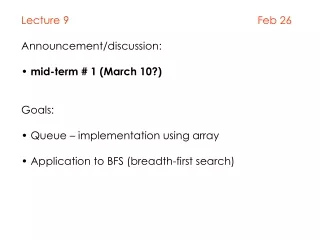
1. Lecture 9 Feb 26 • Announcement/discussion: • mid-term # 1 (March 10?) • Goals: • Queue – implementation using array • Application to BFS (breadth-first search)

2. Queue Overview • Queue ADT • FIFO (first-in first-out data structure) • Basic operations of queue • Insert, delete etc. • Implementation of queue • Array

3. Queue ADT • Like a stack, a queue is also a list. However, with a queue, insertion is done at one end, while deletion is performed at the other end. • Accessing the elements of queues follows a First In, First Out (FIFO) order. • Like customers standing in a check-out line in a store, the first customer in is the first customer served.

4. Insert and delete • Primary queue operations: insert and delete • Like check-out lines in a store, a queue has a front and a rear. • insert - add an element at the rear of the queue • delete – remove an element from the front of the queue Insert Remove front rear

5. Implementation of Queue • Queues can be implemented as arrays • Just as in the case of a stack, queue operations (insertdelete, isEmpty, isFull, etc.) can be implemented in constant time

6. Implementation using Circular Array • When an element moves past the end of a circular array, it wraps around to the beginning, e.g. • OOOOO7963  (insert(4)) 4OOOO7963 • How to detect an empty or full queue, using a circular array? • Use a counter for the number of elements in the queue. • size == MSIZE means queue is full • Size == 0 means queue is empty.

7. Queue Class • Attributes of Queue • front/rear: front/rear index • size: number of elements in the queue • Q: array which stores elements of the queue • Operations of Queue • IsEmpty(): return true if queue is empty, return false otherwise • IsFull(): return true if queue is full, return false otherwise • Insert(k): add an element to the rear of queue • Delete(): delete the element at the front of queue

8. class queue { private: point* Q[MSIZE]; int front, rear, size; public: queue() { // initialize an empty queue front = 0; rear = 0; size = 0; for (int j=0; j < MSIZE; ++j) Q[j] = NULL; } void insert(point* x) { if (size != MSIZE) { rear++; size++; if (rear == MSIZE) rear = 0; Q[rear] = x; }; else cout << “queue is full. Insertion failed” << endl; } point objects have two fields p.x and p.y both of which are int values. (We need a queue to hold the pixel coordinates in project # 3.)

9. point delete() { if (size != 0) { point temp(Q[front]->getx(), Q[front]->gety()); front++; if (front == MSIZE) front = 0; size--; return temp; }; else cout << “attempt to delete from an empty queue” << endl; } bool isEmpty() { return (size == 0); } bool isFull() { return (size == MSIZE); } };

10. Breadth-first search using a queue BFS: application that can be implemented using a queue. Our application involves finding the number of distinct letters that appear in an image and draw bounding boxes around them. Taken from the output of the BFS algorithm

11. Overall idea behind the algorithm Scan the pixels of the image row by row, skipping over black pixels until you encounter a white pixel p(j,k). (j and k are the row and column numbers of this pixel.) Now the algorithm uses a queue Q to identify all the white pixels that are connected together with p(j,k) to form a single symbol/character in the image. When the queue becomes empty, we would have identified all the pixels that form this character (and assigned the color Green to them.) While identifying these connected pixels, also maintain the four variables lowx, highx, lowy and highy. These are the bounding values. When the queue is empty, these bounding values are the x- and y-coordinates of the bounding box.

12. Let the image width be w and the height be h; Set visited[j,k] = false for all j,k; count = 0; Initialize Q;   // count is the number of symbols in the image. for j from 1 to w – 1 do for k from 0 to h – 1 do if (color[j,k] is white) then count++; lowx = j; lowy = k; highx = j; highy = k; insert( [j,k]) into Q; visited[j,k] = true; while (Q is not empty) do p = delete(Q); let p = [x,y];color[x,y] = green; if x < lowx then lowx = x;if y < lowy then lowy = y; if x > highx then highx = x;if y > highy then highy = y; for each neighbor n of p do if visited[n] is not true then visited[n] = true; if (color[n] is white) insert(n) into Q; end if; end if; end for; end while; draw a box with (lowx-1,lowy-1) as NW and (highx + 1, highy + 1) as SE boundary; // make sure that highx+1 or highy+1 don’t exceed the dimensions else visited[j,k] = true;end if; end do; end do;

13. Example: 0 1 2 3 4 5 6 7 0 1 2 3 4 5 6 7

14. Example: when the algorithm stops, count would be 1 xlow = 2 xhigh = 6 ylow = 1 yhigh = 7 Draw the bounding box (2,1), (2,6), (7,1) and (7, 6). 0 1 2 3 4 5 6 7 0 1 2 3 4 5 6 7

15. Example: when the algorithm stops, count would be 1 xlow = 2 xhigh = 6 ylow = 2 yhigh = 7 Draw the bounding box (2,1), (2,6), (7,1) and (7, 6). 0 1 2 3 4 5 6 7 0 1 2 3 4 5 6 7

16. Example: 0 1 2 3 4 5 6 7 count = 0 Q = { } visited changes as shown in fig. 0 1 2 3 4 5 6 7 t t

17. Example: 0 1 2 3 4 5 6 7 count = 1; lowx = highx = 2 lowy = highy = 3 Q = {(2,3)} 0 1 2 3 4 5 6 7 t t t

18. Example: 0 1 2 3 4 5 6 7 0 1 2 3 4 5 6 7 After first Q.delete(): Q = { } count = 1; lowx = highx = 2 lowy = highy = 3 Q = {(3, 3)} t t t t

19. Example: 0 1 2 3 4 5 6 7 After second Q.delete(): Q = { } P = (3,3) color[p] = green lowx = 2 highx = 3 lowy = highy = 3 Q = {(4,3), (3,4)} 0 1 2 3 4 5 6 7 t t t t t t

20. Example: 0 1 2 3 4 5 6 7 After third delete(Q): Q = {(3,4)} P = (4,3) color[p] = green lowx = 2 highx = 4 lowy = highy = 3 Q = {(3,4),(5,3)} 0 1 2 3 4 5 6 7 t t t t t t t

21. Example: After fourth delete(Q): visited[3,4]= true Q = {(5, 3)} P = (3, 4) color[p] = green lowx = 2 highx = 4 lowy = 3 highy = 4 Q = {(5,3),(3,5)} 0 1 2 3 4 5 6 7 0 1 2 3 4 5 6 7 t t t t t t t t

22. Example: After fifth delete(Q): visited[5,3]= true Q = {(3,5)} P = (3, 5) color[p] = green lowx = 2 highx = 5 lowy = 3 highy = 4 Q = {(3,5)} 0 1 2 3 4 5 6 7 0 1 2 3 4 5 6 7 t t t t t t t t

23. Example: After sixth delete(Q): visited[5, 3]= true Q = {} P = (5, 3) color[p] = green lowx = 2 highx = 5 lowy = 3 highy = 5 Q = {(3,6)} 0 1 2 3 4 5 6 7 0 1 2 3 4 5 6 7 t t t t t t t t

24. Example: After seventh delete(Q): visited[3,6]= true Q = { } P = (3,6) color[p] = green lowx = 2 highx = 5 lowy = 3 highy = 6 Q = {(3,7)} 0 1 2 3 4 5 6 7 0 1 2 3 4 5 6 7 t t t t t t t t t

25. Example: After eighth delete(Q): visited[3,7]= true Q = { } P = (3,7) color[p] = green lowx = 2 highx = 5 lowy = 3 highy = 7 Q = { } At this point the while loop ends. 0 1 2 3 4 5 6 7 0 1 2 3 4 5 6 7 t t t t t t t t t t