Consumer Demand Theory II Session Overview
250 likes | 292 Vues
Explore consumer choice, equilibrium interpretation, income effect, and demand curve shifts in this session. Learn the equi-marginal principle and examples through food consumption scenarios. Understand the implications of corner solutions and income-consumption curves.

Consumer Demand Theory II Session Overview
E N D
Presentation Transcript
Consumer Demand Theory II Session 3, EA4th July, 2007Prof. Samar K. Datta
Overview of items intended to be covered in this session • Consumer Choice • Interpretation of consumer equilibrium: Equi-marginal principle • Corner solution • Diminishing MU & diminishing MRS • Income effect and distinction between normal and inferior goods • Engel curve • Price consumption curve and demand curve • Substitutes and complements • Examples /Food for thought
Two conditions for optimal consumer choice 1) Must be located on the budget line. 2) Must give the consumer the most preferred combination of goods and services (i.e., maximum satisfaction).
At market basket A the budget line and the indifference curve are tangent and no higher level of satisfaction can be attained. A At A: MRS =Pf/Pc = .5 U2 Budget Line Consumer Choice Pc= $2 Pf = $1 I = $80 Clothing (units per week) 40 30 20 0 20 40 80 Food (units per week)
When consumers maximize satisfaction: Marginal utility andconsumer choice • Since MRS is also equal to the ratio of the marginal utilities of consuming F and C:
Marginal utility andconsumer choice • The equation for utility maximization can be alternatively expressed as:
Marginal utility andconsumer choice • Total utility is maximized when the budget is allocated so that the marginal utility per dollar of expenditure is the same for each good. • This is referred to as the equal marginal principle.
A corner solution exists at point B. U1 U2 U3 A Corner Solution Frozen Yogurt (cups monthly) A B Ice Cream (cup/month)
Condition for corner solution • MUX/PX > MUY/PY • Implications of corner solution: brand loyalty at any price?
Questions on diminishing MU & diminishing MRS • Does diminishing MRS necessarily imply diminishing MUs? • Does diminishing MUs necessarily imply diminishing MRS?
Income Changes, Income Consumption Curve, and Shift in Demand Curve • Income Changes • An increase in income shifts the budget line to the right,increasing consumption along the income-consumption curve. • Thus, increase in incomeshifts the demand curve to the right.
Income-Consumption Curve 7 D U3 5 U2 B 3 U1 A 4 10 16 Income Consumption Curve Clothing (units per month) Assume: Pf = $1 Pc = $2 I = $10, $20, $30 An increase in income, with the prices fixed, causes consumers to alter their choice of market basket. Food (units per month)
E G H $1.00 D3 D2 D1 4 10 16 Income Changes & Shifts in the Demand Curve Price of food An increase in income, from $10 to $20 to $30, with the prices fixed, shifts the consumer’s demand curve to the right. Food (units per month)
Normal vs. Inferior Good • Normal Good - The income-consumption curve has apositive slope: • The quantity demanded increases with income. • The income elasticity of demand is positive. • Inferior Good - The income-consumption curve has anegative slope: • The quantity demanded decreases with income. • The income elasticity of demand is negative.
15 Income-Consumption Curve Both hamburger and steak behave as a normal good, between A and B... C 10 U3 …but hamburger becomes an inferior good when the income consumption curve bends backward between B and C. B 5 U2 A U1 5 10 20 30 An Inferior Good Steak (units per month) Hamburger (units per month)
Individual Demand • Engel Curves • Engel curves relate the quantity of good consumed to income. • If the good is anormalgood, the Engel curve isupward sloping. • If the good is aninferiorgood, the Engel curve isdownward sloping.
Inferior Engel curve is backward bending for inferior goods. Normal Engel Curves Income ($ per month) 30 20 10 Food (units per month) 0 4 8 12 16
Price Consumption Curve Clothing (units per month) The price-consumption curve traces out the utility maximizing market basket for the various prices for food. 6 A Price-Consumption Curve U1 D 5 B 4 U3 U2 Food (units per month) 4 12 20
Individual Demand relates the quantity of a good that a consumer will buy to the price of that good. E $2.00 G $1.00 Demand Curve $.50 H 4 12 20 Individual Demand Curve Price of Food Food (units per month)
Derivation of Demand Curve from Price Consumption Curve Clothing (units per month) Price of food
Substitutes and Complements • Two goods are consideredsubstitutesif an increase (decrease) in the price of one leads to an increase (decrease) in the quantity demanded of the other. • e.g. movie tickets and video rentals • Two goods are consideredcomplements if an increase (decrease) in the price of one leads to a decrease (increase) in the quantity demanded of the other. • e.g. petrol and motor oil • Two goods areindependentwhen a change in the price of one good has no effect on the quantity demanded of the other.
Substitutes and Complements • Substitutes and Complements • If the price consumption curve isdownward-sloping, the two goods are consideredsubstitutes. • If the price consumption curve isupward-sloping, the two goods are consideredcomplements.
A: Consumption before the trust fund The trust fund shifts the budget line B: Requirement that the trust fund must be spent on education C U3 P C: If the trust could be spent on other goods – i.e., unconstrained B U2 A U1 Q Example: College Trust Fund Other Consumption ($) Education ($)
A With a limit of 2,000 gallons, the consumer moves to a lower indifference curve (lower level of utility). 18,000 D C 15,000 U1 U2 B 2,000 5,000 20,000 Example: Gasoline Rationing Spending on other goods ($) 20,000 Will the consumer be necessarily worse off at D? Gasoline (gallons per year)
Food for thought • How would you display effect of income tax (proportional or progressive) with or without certain exemptions (e.g., on medical insurance)? • How will commodity taxation change consumer equilibrium? • How will income taxation influence labor supply? • How will consumer indifference curves look like if one good is a bad, or both goods are bad? • Is it possible to display exchange between two people having fixed endowments of two goods and no income, when there are no formal markets or prices to facilitate exchange?