Scheduling approaches to MAC
770 likes | 796 Vues
Learn how scheduling approaches optimize packet transfer, reduce delays, and improve throughput in MAC systems. Explore reservation and polling protocols for orderly data transmission.

Scheduling approaches to MAC
E N D
Presentation Transcript
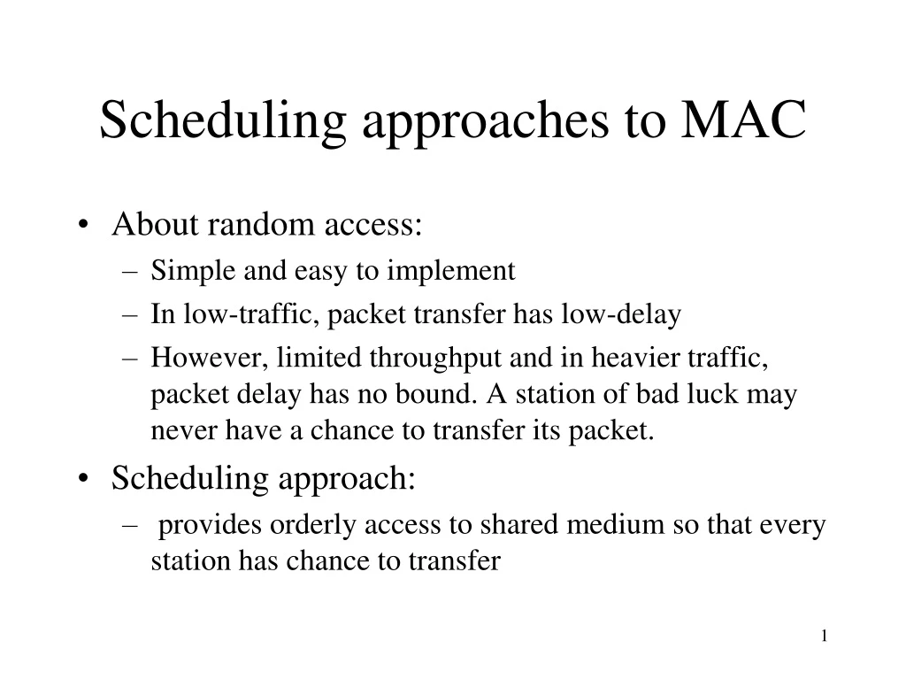
Scheduling approaches to MAC • About random access: • Simple and easy to implement • In low-traffic, packet transfer has low-delay • However, limited throughput and in heavier traffic, packet delay has no bound. A station of bad luck may never have a chance to transfer its packet. • Scheduling approach: • provides orderly access to shared medium so that every station has chance to transfer
Scheduling approach—reservation protocol • The time line has two kinds of periods: • Reservation interval of fixed time length • Data transmission period of variable frames. • Suppose there are M stations, then the reservation interval has M minislots, and each station has one minislot. • Whenever a station wants to transfer a frame, it waits for reservation interval and broadcasts reservation bit in its minislot. • By listening to the reservation interval, every station knows which stations will transfer frames, and in which order. • The stations having reserved for their frame transfer their frames in that order • After data transmission period, next reservation interval begins.
Reservation protocol Frames-transmission Reservation interval 0 1 2 3 4 5 6 7 0 1 2 3 4 5 6 7 1 1 1 1 3 5 1 1 3 7
Scheduling approach—polling protocol • Stations take turns accessing the medium: • At any time, only one station has access right to transfer into medium • After this station has done its transmission, the access right is handed over (by some mechanism) to the next station. • If the next station has frame to transfer, it transfers the frame, otherwise, the access right is handed over to the next next station. • After all stations are polled, next round polling from the station 1 begins.
Centralized polling vs. distributed polling • Centralized polling: a center host which polls the stations one by one • Distributed polling: station 1 will have the access right first, then station 1 passes the access right to the next station, which will passes the access right to the next next station, …
Interaction of polling messages and transmissions in polling systems polling messages … 2 1 4 5 3 M 1 2 t packet transmissions Figure 6.28
Station interfaces: are connected to form a ring by point-to-point lines Stations: are attached to the ring by station interfaces. token Note: point-to-point lines, not a shared bus. Token: a small frame, runs around the ring, whichever gets the token, it has the right to transmit data frames. The information flows in one direction. Station interfaces have important functions. Token-passing rings – a distributed polling network Figure 6.30
Two modes of interface: 1. Listen mode, like a repeater but with some delay, because every arriving bit will be copied into a 1-bit buffer and then copied out. While in the buffer, the bit can be monitored, i.e., inspected and even modified. Therefore, 1-bit delay 2. Transmit mode: transmit frames from its attached station When monitoring, if it finds the passing bits are a data frame with its attached station as destination, then it catches the frame, i.e., copy the bits into its station (may refrain from outputting them). If it finds the passing bits are free token, then if the station has information to send, it will change the token to busy (set one bit to 1) and change to transmit mode. listen mode transmit mode 1 bit delay input from ring output to ring delay to station from station to station from station Token-passing rings – a distributed polling system Figure 6.30
Removing a frame A transmitted frame needs to be removed (absorbed). Who removes it? Choice one: destination station Choice two: transmitting station itself. Choice two is preferred because the destination can insert ACK into the frame and transmitter will get the ACK from its own transmitted frame.
d d d d d d d d d d a). The free token is inserted immediately after the last bit of data frame is sent b). Insert the free token after the last bit of busy token is received c). Insert the free token after the last bit of data frame is received. Generally: when a station seizes the token, it can only transmit limited number of frames or limited time interval to avoid occupying too long. d a) b) c) d d d d Free token Busy token Approaches to token reinsertion: a). multitoken, b). single token, c)single packet Figure 6.31
Comparison of scheduling & random access • Scheduling • Methodical orderly access: dynamic form of time division multiplexing, round-robin (only) when the stations have information to send. • Less variability in delay, supporting applications with stringent delay requirement. In high load, performance is good. E.g., token-ring may reach nearly 100 percent of performance when all stations have plenty of information to send. • Some channel bandwidth carries explicit scheduling information • Random access • Chaotic, unordered access • If rich bandwidth and light load, random access has low delay, otherwise, delay is undeterminably large. • Quite a lot bandwidth is used in collision to alert stations of the presence of other transmissions.
Channelization • Suppose M stations generate steady flow of information • Divide shared medium into M channels so that each station is allocated one channel • Four channelization mechanisms: • FDMA • TDMA • WDMA • CDMA
Time-Division Multiplexing (TDM) (a) Dedicated Lines A1 A2 B1 B2 C1 C2 (b) Shared Line B2 C2 A2 A1 C1 B1 Figure 5.43
1 1 2 MUX MUX 2 . . . . . . 22 23 24 1 b 24 2 b . . . frame 24 24 T-1 carrier system uses TDM to carry 24 digital signals in telephone system Figure 4.4
Frequency-Division Multiplexing (FDM) A f W 0 B f 0 W C B A f C f 0 W (a) Individual signals occupy W Hz (b) Combined signal fits into channel bandwidth Figure 4.2
1 1 2 2 n n Wavelength-division multiplexing (WDM) 1, 2, n MUX deMUX Optical fiber Figure 4.1
CDMA (Code-division multiple access) • Transmissions from different stations occupy entire frequency band at the same time • Different codes are used to separate different transmissions • A code is a unique binary pseudorandom sequence (such as c1,c2,…,cG) (each ci is a +1 or –1 signal) • A binary bit b (i.e., +1 signal) is spread by multiplying it with the code at the sender (which is a sequence of binary information) • At the receiver, the received binary string is multiplied by the same code to get back original bit.
CDMA (cont.) • Since: • b(c1+c2+…+cG) at the sender • The received informationis multiplied by c1,c2,…,cG to get b(c12+c22+…+cG2) = b1=b. • Due to each ci2=1 no matter ci=1 or –1 • So the receiver gets back b. • However, if a different code d1,d2,…,dG is used: • The multiplication will be c1 d1+c2 d2+…+cG dG • Since ci and di are independent, there will be equal number of +1 and –1, so the result will be 0, • Thus the b can not be obtained.
CDMA (cont.) • In order for different codes are randomized, the sequence length G must be long enough. • G is called spreading factor. • Using LSFR (Left-Shift-Feedback-Register).
Transmitter from one user Binary information R1 bps W1 Hz Radio antenna R >> R1bps W >> W1 Hz Unique user binary random sequence Digital modulation CDMA Spread Spectrum Signal • User information mapped into: +1 or -1 for T sec. • Multiply user information by pseudo- random binary pattern of G “chips” of +1’s and -1’s • Resulting spread spectrum signal occupies G times more bandwidth: W = GW1 • Modulate the spread signal by sinusoid at appropriate fc
Binary information Signals from all transmitters Digital demodulation Correlate to user binary random sequence CDMA Demodulation Signal and residual interference • Recover spread spectrum signal • Synchronize to and multiply spread signal by same pseudo-random binary pattern used at the transmitter • In absence of other transmitters & noise, we should recover the original +1 or -1 of user information • Other transmitters using different codes appear as residual noise
g2 g3 g0 Time R0R1R2 0 1 0 0 1 0 1 0 2 1 0 1 3 1 1 0 4 1 1 1 5 0 1 1 6 0 0 1 7 1 0 0 Sequence repeats from here onwards R0 R1 R2 output g(x) = x3 + x2 + 1 The coefficients of a primitive generator polynomial determine the feedback taps Pseudorandom pattern generator • Feedback shift register with appropriate feedback taps can be used to generate pseudorandom sequence
Channelization in Code Space • Each channel uses a different pseudorandom code • Codes should have low cross-correlation • If they differ in approximately half the bits the correlation between codes is close to zero and the effect at the output of each other’s receiver is small • As number of users increases, effect of other users on a given receiver increases as additive noise • CDMA has gradual increase in BER due to noise as number of users is increased • Interference between channels can be eliminated if codes are selected so they are orthogonal and if receivers and transmitters are synchronized • Shown in next example
-1 -1 +1 x x x User 1 + User 2 +1 +1 -1 User 3 Example: CDMA with 3 users • Assume three users share same medium • Users are synchronized & use different 4-bit orthogonal codes: {-1,-1,-1,-1}, {-1,+1,-1,+1}, {-1,-1,+1,+1}, {-1,+1,+1,-1}, Receiver +1 -1 +1 Shared Medium
Channel 1 Channel 2 Channel 3 Sum Signal Sum signal is input to receiver Channel 1:110 -> +1+1-1 -> (-1,-1,-1,-1),(-1,-1,-1,-1),(+1,+1,+1,+1) Channel 2:010 -> -1+1-1 -> (+1,-1,+1,-1),(-1,+1,-1,+1),(+1,-1,+1,-1) Channel 3:001 -> -1-1+1 -> (+1,+1,-1,-1),(+1,+1,-1,-1),(-1,-1,+1,+1) Sum Signal: (+1,-1,-1,-3),(-1,+1,-3,-1),(+1,-1,+3,+1)
x + Example: Receiver for Station 2 • Each receiver takes sum signal and integrates by code sequence of desired transmitter • Integrate over T seconds to smooth out noise Decoding signal from station 2 Integrate over T sec Shared Medium
Sum Signal Channel 2 Sequence Correlator Output +4 Integrator Output -4 -4 Decoding at Receiver 2 Sum Signal: (+1,-1,-1,-3),(-1,+1,-3,-1),(+1,-1,+3,+1) Channel 2 Sequence:(-1,+1,-1,+1),(-1,+1,-1,+1),(-1,+1,-1,+1) Correlator Output:(-1,-1,+1,-3),(+1,+1,+3,-1),(-1,-1,-3,+1) Integrated Output: -4, +4, -4 Binary Output: 0, 1, 0 X =
0 0 0 1 0 0 0 1 0 0 0 1 Wn Wn Wn Wnc W1= 0 W2= W4= W2n= 0 0 0 1 1 1 1 0 0 0 0 1 0 0 0 1 1 1 1 0 0 0 0 1 1 1 1 0 0 0 0 1 0 0 0 1 0 0 0 1 0 0 0 1 0 0 0 1 1 1 1 0 0 0 0 1 1 1 1 0 1 1 1 0 0 0 0 1 1 1 1 0 W8= Walsh Functions • Walsh functions are provide orthogonal code sequences by mapping 0 to -1 and 1 to +1: each row is a code, rows are orthogonal. • Walsh matrices constructed recursively as follows:
LAN bridges • Repeater: used to connect two or more networks at physical layer • Bridge: used to connected two or more networks at data link or MAC layer • Router: used to connect two or more networks at network layer • Gateway: connect two or more networks at higher layers.
LAN bridges’ functions • Bridges are generally used to connect LANs by • Extending a LAN which reach saturation, called bridged/extended LAN • Connect different departments’ LANs, these LANs • Use different network layer protocols, bridges are fine because bridges operate at data link layer which supports different network layer protocols • Located in different building, bridges are fine because bridges can be connected by point-to-point link • Are different LANs: bridges need to have ability to convert between different frame format • Security is big problem in LAN, why? • So bridges need to have some ability of dealing with security issue such as filtering frames, controlling flow of frames in and out. • Bridge is better than repeater when connect two exact same LANs because bridge has the ability to reduce traffic by confining local traffic. • Bridge will monitor MAC address of frames so it can not be in physical layer • Bridge have no routing ability so it is not in network layer.
Bridges generally connect the same types of LANs, so they generally operate at MAC layer. Network Network Bridge LLC LLC MAC MAC MAC MAC Physical Physical Physical Physical Interconnection by a bridge Figure 6.80
A bridged LAN Port #1 Port #2 Figure 6.79
Three type bridges • Transparent bridges: means that stations are completely unaware of the presence of bridges. Used in Ethernet LANs. No burden in stations, bridges take care of all connection related functions. • Source routing bridge: used in token-ring and FDDI LANs. Burden on stations. Source station needs to give route to the destination. Bridges just forward frames based on the route in the frame. • Mixed-media bridges: used to interconnect LANs of • different types. These bridges have abilities of converting • between LANs.
Transparent bridges • Three basic functions: • Forwards frames from one LAN to another • Learns where stations are attached to the LAN • Prevents loops in the topology • A transparent bridge is configured in “promiscuous” mode
Forwarding and forwarding table of bridges • Port is a physical interface, a bridge have two or more ports • For every station in bridged LAN, the port number indicates • which part (direction) of the bridge this station is attached to. • When a frame comes to a bridge, the bridge will forward to the • port corresponding to the MAC address in the table, which is the • destination physical address in the frame. • 4. Question: how to establish forwarding table? No, automatically set up by self learning Manually set up by administrator. Good?
Bridge learning When a bridge receives a frame, it searches through the forwarding table: 1. For source address, if not found, adds source address along coming port # into table 2. For destination address, if found, forwards the frame to the corresponding port, except the corresponding port # being same as the coming port # 3. otherwise (not found), floods the frame to all ports except the coming port
S5 S1 S2 S3 S4 1.S1->S5 2.S3->S2 3.S4->S3 4.S2->S1 LAN1 LAN2 LAN3 Bridge1 Bridge 2 port 1 port 2 port 1 port 2 Address Port Address Port S1 1 S1 1 S3 2 1 S3 2 S4 S4 2 S2 1 Any problem with it? Figure 6.85
LAN topology is dynamic Life is never static in real world. The bridged LAN change constantly. Add station: Easy, learn again. Move station: When find same MAC address, but coming from a different port, update the port number. Timer, associate every entry (a station) in forwarding table a timer, when timer times out, remove the entry from the table. Moreover, when receiving a frame with a source MAC address, if its entry is already in the table, then refresh the timer. Remove station: Any more problem?
Loop in the topology will cause flooding forever S5 S1 S2 S3 S4 S1->S5 LAN1 LAN2 LAN3 Bridge1 Bridge 2 port 1 port 2 port 1 port 2 Bridge3 Figure 6.85
Spanning tree to break loop • Main idea: maintain a spanning tree to include all stations but disable some ports automatically. Thus, remove loop. • Assumptions: unique LAN IDs, unique bridge IDs, and unique port IDs. The lowest ID is used to break a tie.
Steps of spanning tree • Select a root bridge which is the bridge with the lowest bridge ID. • For each bridge except the root bridge, determine the root port which is the port with least-cost path (& lowest ID) to root bridge. • For each LAN, select a designated bridge, which is the bridge offering the least-cost path (& lowest ID) from the LAN to root bridge. The port connecting the LAN and the designated bridge is called a designate port. • All root ports and designated ports are put into forwarding table. These are only ports that are allowed to forward frames. The other ports are placed into a “blocking” state.
LAN1 (1) (1) B1 B2 (2) B3 LAN2 B4 LAN3 B5 LAN4 (1) (2) (3) (2) (1) (2) (1) (2) Figure 6.86
Source routing bridges • Putting burden on end stations, bridges are mainly responsible for forwarding. • Each station determines the route to the destination and put the routing information in the header of the frame. • Source routing information is inserted only when source and destination are in different LANs and is indicated by I/G bit in source address.
Frame format for source routing • Control field contains type of frame, routing information and length of it. 2. Designator contains a 12-bit LAN number and a 4-bit bridge number 3. The highest bit in source address indicates whether it is source routing. Routing Route Route Route Control Designator-1 Designator-2 Designator-m 2 bytes 2 bytes 2 bytes 2 bytes Destination Routing Source Data FCS Address Information Address Question: how to find the route in the first place? Figure 6.88
Mixed-media bridges • Such as connect Ethernet and token-ring networks • Convert between two address representations • Ethernet has maximum size of 1500 bytes but token-ring has no explicit limit. Drop frame if it is too long because bridges do not do segmentation • Token-ring has three status bits A, C and E, but no these bits in Ethernet, so no conversion for them • Different transmission rate, so bridges need buffer to store extra frame temporarily.
IEEE LAN standards • 802.2 LLC • 802.3 CSMA-CD (I.e., Ethernet) • Frame length 64 –1518 (or client data: 46—1500) • 802.4 token-bus • 802.5 token-ring • FDDI (Fiber Distributed Data Interface) • 802.11 wireless networks
Ethernet --history • 1970s, Robert Metcalfe etc. Xerox, connecting workstations • 1980s, DEC, Intel, Xerox, “DIX” Ethernet standard 10Mpbs • The basis for IEEE 802.3 standard, “thick” coaxial cable in 1985. • 802.3 and “DIX” Ethernet differ in one header field definition. • Expended to “thin” coaxial, twisted-pair, optical fiber. • 1995: 100Mbps, 1998: 1Gbps, 2002: 10Gbps.
Ethernet -- basis • Bus based coaxial cable • CDMA-CD with 1-persistent • Minislot time: two propagation delays • 10Mbps, 2500 meters, 4 repeaters • (Truncated) binary exponential backoff algorithm • Three periods and performance
Ethernet --backoff • (Truncated) binary exponential backoff algorithm • Whenever collision, wait for B minislots • B is determined as followed: • After 1th collision, B is selected from 0 to 1 • After 2th collision, B is selected from 0 to 3 • After 3th collision, B is selected from 0 to 7 • … • After nth collision, B is selected from 0 to • 2n-1 if n<10 and 210-1 if n<=16, otherwise, give up.