Download
1 / 41
460 likes | 721 Vues
AMR Simulations of the Magneto-hydrodynamic Richtmyer-Meshkov Instability. Ravi Samtaney Computational Plasma Physics Group Princeton Plasma Physics Laboratory Princeton University CPPG Seminar PPPL, 04/09/2003. Acknowledgement. Phillip Colella and Applied Numerical Algorithms Group, LBNL

E N D
AMR Simulations of the Magneto-hydrodynamic Richtmyer-Meshkov Instability Ravi Samtaney Computational Plasma Physics Group Princeton Plasma Physics LaboratoryPrinceton University CPPG SeminarPPPL, 04/09/2003
Acknowledgement • Phillip Colella and Applied Numerical Algorithms Group, LBNL • Steve Jardin, PPPL • DOE SciDAC program
Outline • MHD primer (MHD with shocks) • Richtmyer-Meshkov Instability (RMI) • RMI suppression in MHD • Numerical Method • Adaptive Mesh Refinement (AMR) • Unsplit upwinding method • div(B) issues • Conclusion and future work
Electromagnetic Coupling • Weakly coupled formulation • Hydrodynamic quantities in conservative form, electrodynamic terms in source term • Hydrodynamic conservation & jump conditions • One characteristic wave speed (ion-acoustic) • Tightly coupled formulation • Fully conservative form • MHD conservation and jump conditions • Three characteristic wave speeds (slow, Alfvén, fast) • One degenerate eigenvalue/eigenvector j¢ E
Single-fluid resistive MHD Equations • Equations in conservation form Parabolic Hyperbolic Reynolds no. Lundquist no. Peclet no.
MHD Discontinuities • MHD shock waves • Fast shocks • Slow shocks • Intermediate shocks (unstable if =0) • Compound shocks (shock-rarefaction structures do not occur in ideal MHD) • Alfvén shocks • MHD contact discontinuities • No tangential jump in velocity if normal component of B is present • Shear flow discontinuities allowed if B.n=0 Figures from PhD thesis of Hans De Sterck, Katholieke Universiteit Leuven
h l g(t) = constant (RT) = U (t) (RM) Growth rate of perturbation: Exponential (RT) Linear (RM) Richtmyer-Meshkov Instability (RMI) • RMI • occurs at a fluid interfaceaccelerated by a shock-wave • “impulsive Rayleigh-Taylor” • Linear stability analysis by Richtmyer (1960) • Experimental confirmation by Meshkov (1970)
Richtmyer-Meshkov Instability (RMI) • Occurs • in inertial confinement fusion where it is the main inhibiting hydrodynamic mechanism • in astrophysical situations • Approx. 200 peer-reviewed publications + numerous proceedings in last 15 years. X-ray images from Nova laser expts.Barnes et al. (LANL Progress Report 1997)
Parameters and Initial/Boundary Conditions • Parameters which completely define the posed Mathematical problem • Mach number of the incident shock, M • Density ratio (or Atwood number at the fluid interface), , At=(-1)/(+1) • Perturbation • Magnetic field strength -1=B02/2p0
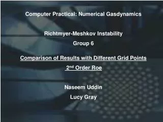
Simulation Results • Parameters which completely define the posed M=2, =45o, =3, -1=0 (B0=0) or-1=0.5 (B0=1) t=0.385
Simulation Results • t=1.86
Simulation Results • t=3.33 “Results! Why, man, I have gotten a lot of results. I know severalthousand things that won’t work”- Thomas Edison
=0 in 2D zero during incidentshock refraction phase Baroclinic source Vortex Dynamical Interpretation • During incident shock refraction on the density interface vorticity is generated due to misalignment of density and pressure gradients (Hawley and Zabusky, PRL 1989) Light Heavy r p r p Heavy Light r r
Why does B suppress the instability? – A mathematical explanation • Consider jump conditions across a stationary discontinuity[ un] = 0[ un2 + p + ½ B2 – ½ Bn2] = 0[ un ut – Bn Bt ] = 0[Bn] = 0[Bt un – Bn ut] = 0[(e + p + ½ B2) un – Bn (u¢ B)] =0 • For un=0 (no flow through discontinuity) implies • [ut] = 0 if Bn!=0 or • [p+Bt2] = 0 and ut and Bt can jump if Bn=0 • For un!=0, ut jumps across the discontinuity. • In MHD shocks can support shear • Jump conditions originally derived by Teller and do Hoffman (1952) Other sources: Friedrichs and Kranzer (1958), Anderson (1963) “Young man, in mathematics you don’t understand things, you just get used to them” – J. Von Neumann
Vortex sheets – Early Refraction Phase • t=0.385 • The shocked interface is a vortex sheet (-1=0) • In MHD shocks can support shear
Vortex Dynamical Interpretation • Baroclinic vorticity is taken away by slow shocks in the presence of a magnetic field. These shocks are stable (at least in our simulations) • Net circulation in the domain
Current Sheets – Early Refraction Phase • t=0.385
t=1.91 RF TF t=3.31 RS TS I don’t believe this! What if B is really small? • In case the magnetic field is very small, the slow shocks move closer to the interface. The interface amplitude grows due to an “entrainment” effect. -1=0.05
Results for < 1 t=1.91 • The same suppression effect is observed t=3.31
Adaptive Mesh Refinement • Adaptive mesh refinement provides a “numerical microscope” • Provides resolution where we need it • Optimally should be based on a local truncation error analysis • Mesh refined where local error exceeds a user defined threshold • In practice, we refine the mesh where a threshold is exceeded (usually depends on gradients of flow quantities) • LTE analysis is not very meaningful if discontinuities are present • Usually leads to more efficient compuations • Various AMR frameworks/packages • GrACE • SAMRAI • Paramesh • CHOMBO • AMRITA
Why AMR? • For the RMI case • Base mesh 256x32 • Plus 3 levels of refinement (each with a factor of 4) • Effective uniform mesh of 16384x 2048 • Estimated computational saving about a factor of 25 • Each run took about 80 hours on NERSC • Uniform mesh run would have taken 25x80=2000 hours • % Area covered • Finest mesh: 2.1% • Level 2 : 6.5% • Level 1 : 15.6% “ It is unworthy of excellent mento lose hours, like slaves, in thelabors of calculation” -Gottfried Wilhelm Leibnitz
Why AMR? • Area covered • Finest mesh (321) : 7.6 % • Level 2 (38): 18.5% • Level 1 (5): 50 % • Level 0 (2): 100 %
Layer of ghost cells AMR Basics • Flag cells which need to be refined • Using a clustering algorithm make patches • Copy from previous overlapping fine mesh and interpolate from coarse mesh where new refinement occurs • Surround each fine patch with a layer of ghost cells • Interpolation must be consistent to the order of the method
Coarse at tn+1 Fine at tn+1 Fine at tn+1/2 Coarse at tn Fine at tn AMR Basics • Update coarse mesh solution • Update fine mesh “r” times • Coarse mesh solution interpolated in space and time to provide boundary conditions at CFI • Synchronize at the end of each time step by flux refluxing to maintain strong conservation • Average fine mesh solution replaces coarse solution where coarse/fine meshes overlap Adaptive time stepping Synchronizeby replacingcoarse meshfluxes by fine mesh fluxes at CFI
Adaptive Mesh Refinement with Chombo • Chombo is a collection of C++ libraries for implementing block-structured adaptive mesh refinement (AMR) finite difference calculations (http://www.seesar.lbl.gov/ANAG/chombo) • (Chombo is an AMR developer’s toolkit) • Mixed language model • C++ for higher-level data structures • FORTRAN for regular single grid calculations • C++ abstractions map to high-level mathematical description of AMR algorithm components • Reusable components. Component design based on mathematical abstractions to classes • Based on public-domain standards • MPI, HDF5 • Chombovis: visualization package based on VTK, HDF5 • Layered hierarchical properly nested meshes • Adaptivity in both space and time
Chombo Layered Design • Chombo layers correspond to different levels of functionality in the AMR algorithm space • Layer 1: basic data layout • Multidimensional arrays and set calculus • data on unions of rectangles mapped onto distributed memory • Layer 2: operators that couple different levels • conservative prolongation and restriction • averaging between AMR levels • interpolation of boundary conditions at coarse-fine interfaces • refluxing to maintain conservation at coarse-fine interfaces • Layer 3: implementation of multilevel control structures • Berger-Oliger time stepping • multigrid iteration • Layer 4: complete PDE solvers • Godunov methods for gas dynamics • Ideal and single-fluid resistive MHD • elliptic AMR solvers
Numerical Method: Upwind Differencing • The “one-way wave equation” propagating to the right: • When the wave equation is discretized “upwind” (i.e. using data at the old time level that comes from the left the wave equations becomes: • Advantages: • Physical: The numerical scheme “knows” where the information is coming from • Robustness: The new value is a linear interpolation between two old values and therefore no new extrema are introduced
Symmetrizable MHD Equations • The symmetrizable MHD equations can be written in a near-conservative form (Godunov, Numerical Methods for Mechanics of Continuum Media, 1, 1972, Powell et al., J. Comput. Phys., vol 154, 1999): • Deviation from total conservative form is of the order of B truncation errors • The symmetrizable MHD equations lead to the 8-wave method. The eigenvalues are • The fluid velocity advects both the entropy and div(B)in the 8-wave formulation
Numerical Method: Finite Volume Approach • Conservative (divergence) form of conservation laws: • Volume integral for computational cell: • Fluxes of mass, momentum, energy and magnetic field entering from one cell to another through cell interfaces are the essence of finite volume schemes. This is a Riemann problem.
Numerical method: Riemann Solver • The eigenvalues and eigenvectors of the Jacobian, dF/dU are at the heart of the Riemann solver: • Each wave is treated in an upwind manner • The interface flux function is constructed from the individual upwind waves • For each wave the artificial dissipation (necessary for stability) is proportional to the corresponding wave speed • Discontinuous initial condition • Interaction between two states • Transport of mass, momentum, energy and magnetic flux through the interface due to waves propagating in the two media • Riemann solver calculates interface fluxes from left and right states
-U t A3 A1 A4 A2 Unsplit method – Basic concept • Original idea by P. Colella (Colella, J. Comput. Phys., Vol 87, 1990) • Consider a two dimensional scalar advection equation • Tracing back characteristics at t+ t • Expressed as predictor-corrector • Second order in space and time • Accounts for information propagating across corners of zone Corner coupling I II
Unsplit method: Hyperbolic conservation laws • Hyperbolic conservation laws • Expressed in “primitive” variables • Require a second order estimate of fluxes
Unsplit method: Hyperbolic conservation laws • Compute the effect of normal derivative terms and source term on the extrapolation in space and time from cell centers to cell faces • Compute estimates of Fd for computing 1D Flux derivatives Fd / xd - I + I
Unsplit method: Hyperbolic conservation laws • Compute final correction to WI,§,d due to final transverse derivatives • Compute final estimate of fluxes • Update the conserved quantities • Procedure described for D=2. For D=3, we need additional corrections to account for (1,1,1) diagonal couplingD=2 requires 4 Rieman solves per time stepD=3 requires 12 Riemann solves per time step II
The r¢ B=0 Problem • Conservation of B =0: • Analytically: if B =0 at t=0 than it remains zero at all times • Numerically: In upwinding schemes the curl and div operators do not commute • Approaches: • Purist: Maxwell’s equations demand B =0 exactly, so B must be zero numerically • Modeler: There is truncation error in components of B, so what is special in a particular discretized form of B? • Purposes to control B numerically: • To improve accuracy • To improve robustness • To avoid unphysical effects (Parallel Lorentz force)
Approaches to address the r¢B=0 constraint • 8-wave formulation: r¢ B = O(h) (Powell et al, JCP 1999; Brackbill and Barnes, JCP 1980) • Constrained Transport (Balsara & Spicer JCP 1999, Dai & Woodward JCP 1998, Evans & Hawley Astro. J. 1988) • Field Interpolated/Flux Interpolated Constrained Transport • Require a staggered representation of B • Satisfy r¢ B=0 at cell centers using face values of B • Constrained Transport/Central Difference (Toth JCP 2000) • Flux Interpolated/Field Interpolated • Satisfy r¢ B=0 at cell centers using cell centered B • Projection Method • Vector Potential (Claim: CT/CD schemes can be cast as an “underlying” vector potential. Evans and Hawley, Astro. J. 1988) • Require ad-hoc corrections to total energy • May lead to numerical instability (e.g. negative pressure – ad-hoc fix based on switching between total energy and entropy formulation by Balsara)
r¢B=0 by Projection • Compute the estimates to the fluxes Fn+1/2i+1/2,j using the unsplit formulation • Use face-centered values of B to compute r¢ B. Solve the Poisson equation r2 = r¢ B • Correct B at faces: B=B-r • Correct the fluxes Fn+1/2i+1/2,j with projected values of B • Update conservative variables using the fluxes • The non-conservative source term S(U) r¢ B has been algebraically removed • On uniform Cartesian grids, projection provides the smallest correction to remove the divergence of B. (Toth, JCP 2000) • Does the nature of the equations change? • Hyperbolicity implies finite signal speed • Do corrections to B via r2=r¢ B violate hyperbolicity? • Conservation implies that single isolated monopoles cannot occur. Numerical evidence suggests these occur in pairs which are spatially close. • Corrections to B behave as 1/r2 in 2D and 1/r3 in 3D • Projection does not alter the order of accuracy of the upwinding scheme and is consistent
Unsplit + Projection AMR Implementation • Implemented the Unsplit method using CHOMBO • Solenoidal B is achieved via projection, solving the elliptic equation r2=r¢ B • Solved using Multgrid on each level (union of rectangular meshes) • Coarser level provides Dirichlet boundary condition for • Requires O(h3) interpolation of coarser mesh on boundary of fine level • a “bottom smoother” (conjugate gradient solver) is invoked when mesh cannot be coarsened • Physical boundary conditions are Neumann d/dn=0 (Reflecting) or Dirichlet • Multigrid convergence is sensitive to block size • Flux corrections at coarse-fine boundaries to maintain conservation • A consequence of this step: r¢ B=0 is violated on coarse meshes in cells adjacent to fine meshes. • Code is parallel • Second order accurate in space and time
Conclusion (These, gentlemen, are the opinions upon which I will base my facts” – Winston Churchill) • Numerical evidence presented that the RMI is suppressed in the presence of a magnetic field • Mathematical explanation • Physical explanation still lacking • Conjectures: Main result will remain essentially same • For non-ideal MHD • For Hall MHD • In three dimensions • A conservative solenoidal B AMR MHD code was developed • Unsplit upwinding method for hyperbolic fluxes • r¢ B=0 achieved via projection (“If the facts don’t fit the theory, change the facts”- Albert Einstein)
Related AMR Work • High resolution parallel 2D magnetic reconnection runs. • Implicit treatment of viscous/conductivity terms • Pellet injection AMR simulations