CHAPTER 21 CONSUMPTION AND INVESTMENT
281 likes | 808 Vues
CHAPTER 21 CONSUMPTION AND INVESTMENT. The Life Cycle Hypothesis. Life Cycle Hypothesis.

CHAPTER 21 CONSUMPTION AND INVESTMENT
E N D
Presentation Transcript
CHAPTER 21CONSUMPTION AND INVESTMENT The Life Cycle Hypothesis
Life Cycle Hypothesis “the saving and consumption decisions of households at each point of time reflect a more or less conscious attempt at achieving the preferred distribution of consumption over the life cycle, subject to the constraint imposed by the resources accruing to the household over its lifetime” by Franco Modigliani, Albert Ando, Richard Brumberg (1963) A household’s consumption depends on current income and long-term expected income. Expenditures are planned based on expected earnings over their lifetime.
www.economyprofessor.com Life cycle hypothesis was developed by: American economist Irving Fisher (1867-1947) English economist Roy Harrod (1900-1978) Japanese economist Albert Ando (1929-2001) Italian-born economist Franco Modigliani (1918-2003). “individuals consume a constant percentage of the present value of their life income, dictated by preferences and tastes and income.” ANDO and Modigliani: - APC is higher in young and old households - APC is lower for middle-aged people
Consumption Function “individuals consume a constant percentage of the present value of their life income” 1 T x = Expected lifetime resources Consumption in period t T = additional years of life expectancy Yt1 = current labor income N = expected years to retirement Y1e = average expected annual labor income over N-1 years At = value of present assets
Changes in current income When only current income, Yt, changes, then C will change by 1/T: But when changes in current income, Yt1, also affects the average expected future income, Y1e, then Y1e changes, and C will change by 1/T plus (N-1)/T: +
Scenario A 30-year old worker who has a life expectancy of 80 years, plans to retire in 40 years’ time. What is his T value? 80 – 30 = 50 (years more to live) What is his retirement age? 30 + 40 = 70 (works for 40 more years) How many years of retirement? 80 – 70 = 10 (retires at 70, dies at 80) Assumptions: Constant consumption flow. Consume all before expected life’s end. No interest paid on assets. Saving = future consumption.
Transient change ΔYt1 A $100 one-time increase in current income will result in a $2 increase in C every year. (This worker will still be working for another 40 years and following which, he will retire for another 10 years. So the one-time additional $100 is being distributed as additional $2 consumption every year for the next 50 years.) When only his current income changes, his C will change by:
Permanent change ΔYt1e When changes in current income also changes the average expected future income, his C will change by: A $100 permanent increase in current income will result in a $80 increase in C every year. (This worker will work for 40 years and receive additional $100 in annual salary. But his C will only increase by $80 each year. He will save $20 every year until he retires. His savings will be $20 x 40 years = $800. When he retires at age 70, he will receive additional $80 for 10 years from his savings that he will use for C.)
Life Cycle Consumption, C Time Young: Started working High spending Loans/Dissaving Income, Y • Middle-age: • Stable job • Low spending • High saving • Retiree: • Less/no income • High spending • Dissaving
Aggregate C Function Aggregate consumption depends on: From Ando & Modigliani: If Y1e is a multiply of Yt1, then Y1e = βYt1 where β>0. current labor income average future expected labor income wealth becomes
Estimates An increase in current income of $100 with the assumed effect on future labor income will increase consumption by $72. An increase in wealth of $100 will increase consumption by $72. From Ando & Modigliani, Ct = 0.72 Yt1 + 0.06At ** When changes in current income does not affect expected future income (i.e. transient or temporary rise in salary), then an increase in current income of $100 will increase consumption by $6 (whereby b1 has the same value as b3, and b1 is also the MPC).
Short-run Concumption, C Life cycle hypothesis explains that in the short-run, the relationship between C and YD can be nonproportional, C = a + bYD whereby constant a represents the effect of wealth. i.e. Ct = 0.06At + 0.72 Yt1where 0.06At is the intercept. As the level of wealth increases over time, short-run C will move upwards. SCF2 SCF1 Disposable income, YD SCF0
Long-run Concumption, C at Ct = 0.06At + 0.72Yt1; where At = 4.75YD, Yt1 = 0.88YD; then aggregate consumption is: Ct = 0.06 (4.75YD) + 0.72(0.88YD) Ct = 0.92YD MPC = APC = Ct / YD = 0.92 LCF Life cycle hypothesis also explains that in the long-run, the relationship between C and YD tend to become proportional, C = bYD whereby the slope, MPC, which, without intercept, is equals to APC. Disposable income, YD
Income Level In the Family Budget study, - APC of the families with a higher level of income is very low, their APS is very high - APC of the families with a lower level of income is very high, their APS is very low Life cycle hypothesis explains that people with higher level of income are mostly in the “middle-age” life range in which they hold stable jobs and therefore tend to save more than they spend. Whereas people with lower level of income are mostly young individuals who has just started working and elderly people who has already retires and has no income, hence their tendency to spend more than they can save.
Quarterly Movements In the quarter-to-quarter study, results were inconclusive a mix of different response to increase in income Life cycle hypothesis explains that this could be due to one-time increase in current income, hence no permanent effect on consumption. Transient changes alters the consumer behavior for the period in which the any one factor influences their consumption.
Liquidity Constraints Critics of Life Cycle Hypothesis: - Life cycle hypothesis neglects the importance of liquidity constraints. (Flavin, 1981, 1985 shows significance of liquidity constraints) - Young people may have difficulties attaining “loans” to finance their high consumption. - Accumulated assets owned by the retirees may not be “liquid” to care for their retirement years. - People may actually want to save more for bequests/ inheritance rather than saving for own consumption in retirement years. (Kotlikoff & Summers, 1981, supports bequests as motive for savings)
Policy Implications Ct = 0.06At + 0.72 Yt1 Fiscal policy: any permanent or long-term policy changes that affect current income will also affect the expected lifetime income. any transient or short-term policy changes that may alter the liquidity constraints of consumers’ assets may also affect the expected lifetime income. Monetary policy: policies that affect investment decisions will affect consumers’ wealthand asset liquidity tight monetary policy high liquidity constraints, less C expansionary monetary policy low liquidity constraints, more C
Conclusion • A household’s consumption depends on current income and long-term expected income. Expenditures are planned based on expected earnings over their lifetime. • ANDO and Modigliani: APC is higher in young and old households, lower for middle-aged people • Short-run, the relationship between C and YD can be nonproportional, C = a + bYD whereby constant a represents the effect of wealth. • Long-run, the relationship between C and YD tend to become proportional, C = bYD whereby the slope, MPC equals to APC. • Quarterly movement may due to one-time (transient) increase in current income, hence no permanent effect on consumption. • Critics: life cycle hypothesis does not explain liquidity constraints. • Fiscal policy may affect C via taxes on current income, monetary policy via interest rate and investment decisions.