Comprehensive Scheduling Model for Job Processing in Manufacturing
This comprehensive guide focuses on modeling scheduling parameters essential for efficient job processing in manufacturing settings. It outlines key aspects such as resource configurations, job processing times, release dates, and constraints like precedence, routing, and resource capabilities. It also discusses objective functions and performance measures, including throughput and makespan, while considering both deterministic and stochastic scheduling models. The text emphasizes optimizing production through various cutting-edge scheduling strategies and dynamic problem-solving techniques.

Comprehensive Scheduling Model for Job Processing in Manufacturing
E N D
Presentation Transcript
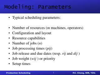
Modeling: Parameters • Typical scheduling parameters: • Number of resources (m machines, operators) • Configuration and layout • Resource capabilities • Number of jobs (n) • Job processing times (pij) • Job release and due dates (resp. rij and dij ) • Job weight (wij ) or priority • Setup times
Modeling: Objective function • Objectives and performance measures: • Throughput, makespan (Cmax, weighted sum) • Due date related objectives (Lmax, Tmax, ΣwjTj) • Work-in-process (WIP), lead time (response time), finished inventory • Total setup time • Penalties due to lateness (ΣwjLj) • Idle time • Yield • Multiple objectives may be used with weights
Modeling: Constraints • Precedence constraints (linear vs. network) • Routing constraints • Material handling constraints • (Sequence dependent) Setup times • Transport times • Preemption • Machine eligibility • Tooling/resource constraints • Personnel (capability) scheduling constraints • Storage/waiting constraints • Resource capacity constraints
Machine configurations: • Single-machine vs. parallel-machine • Flow shop vs. job shop Processing characteristics: • Sequence dependent setup times and costs • length of setup depends on jobs • sijk: setup time for processing job j after k on machine i • costs: waste of material, labor • Preemptions • interrupt the processing of one job to process another with a higher priority
Generic notation of scheduling problem • Machine Job Objective • characteristics characteristics function • for example: • Pm | rj, prmp | ΣwjCj (parallel machines) • 1 | sjk | Cmax (sequence dependent • setup / traveling salesman) • Q2 | prec | ΣwjTj (2 machines w. different speed, precedence rel., weighted tardiness)
Scheduling models • Deterministic models • input matches realization • vs. • Stochastic models • distributions of processing times, release and due dates, etc. known in advance • outcome/realization of distribution known at completion
Static V.S. Dynamic • Static Assume all the jobs are ready at the beginning which means ai=0 • Dynamic Each job with a different arrival time. Which ai≠0
Large Scale Problem (man-made) approach Upper Bound (Heuristic) available solution space Optimum unavailable solution space Lower Bound (Release Constraints) approach
Performance Measure • Max Completion Time (Makspan) • Cmax = Max Ci = C6 • Minimize Inventory • fi : Reduce Inv. • fi = Ci – ai ( Static Problem : ai=0) • Satisfy Due Date • Tardiness = Max(Ci-di , 0 ) • Earliness = Max(di-Ci , 0 ) • JIT = Ci-di • Bi-criteria Multi-Objective (flow time = waiting time + process time)
1 2 3 4 0 5 8 12 13 Compute flow time 5 3 4 1 5 5 5 5 3 3 3 4 4 1
Gantt Chart 3 2 1 5 4 6 jobs are ready d3 c3d1c2 d2 c1d4c5c4d5 d6 = c6 flow time tardiness c2 – a2 c4 > d4
Scheduling Problem Representation 4 / 1 / (n / m / o ) objective function # machine # job . . . . .
Example: A factory has receive 4 different orders as follows • Please assign the production sequence of the 4 jobs to satisfy: • Due Date • Min Inventory
Sol. 1. Using FCFS (First come first serve) 1-2-3-4 1 2 3 4 0 5 8 12 13
Sol. • Using EDD (Earliest Due Date) 4-2-3-1 4 2 3 1 0 1 4 8 13
Sol. • Using SPT (Shortest Processing Time) The same with EDD Optimum 4-2-3-1 4 2 3 1 0 1 4 8 13 • EDD – Due Date – Tmax • SPT – Inventory - Flow time
Bi-criterion SPT Frontier EDD
HW. 5 / 1 / Draw the Frontier when
Dynamic Problem Example: 4 / 1 /
Sol. Ck > ai , C1≧ a2 - no idle time Else, if ai > Ck, a2 > C1 - idle 1. Using Job index 1-2-3-4 1 2 3 4 0 3 8 11 15 16 3-5 3-2 3-4 • 5-2 5+1 5-1 =18 • 3 3 3 = 9 • 4 4 = 8 • 1 = 1 • 36 or
Sol. 2. Using SPT. EDD 4-2-3-1 4 2 3 1 0 4 5 8 12 17
Sol. 3. Using FCFS then SPT (ESPT) Use SPT to arrange jobs (available jobs) 3-4-2-1 3 4 2 1 0 2 6 7 10 15 Static (SPT) After arrange job 3, the dynamic problem will become a Static one. Then use SPT.
Ex:ESPT • find Min • for min
Sol. 1. Using Job index 1-2-3-4 1 2 3 4 0 3 8 11 15 16
Sol. • Using SPT • Using EEDD (next slide) 4-2-3-1 4 2 3 1 0 4 5 8 12 17
Ex:EEDD • find Min • for min let • Return 3
JIT problem Slackness Rule: Find di-pi (Job j have to start before this time) a4 d4 a2 d2 a3 d3 a1 d1 2 4 1 3 try 2 1 2 or
Ex. 2-4-3-1 2 4 3 1 0 5 9 10 17 26
HW. 1. 5 / 1 / 2. 5 / 1 / 3. 5 / 1 / Find an optimal solution!