Download

1 / 54
540 likes | 711 Vues
Connectivity Verification in VLSI Layout. Shmuel Wimer Bar Ilan Univ., School of Engineering. Outline. Modeling connectivity Finding connected components in graphs Directed graphs by DFS Non directed graphs by UNION_FIND Intersection of rectangles Interval Tree Priority search tree

E N D
Connectivity Verification in VLSI Layout Shmuel Wimer Bar Ilan Univ., School of Engineering
Outline • Modeling connectivity • Finding connected components in graphs • Directed graphs by DFS • Non directed graphs by UNION_FIND • Intersection of rectangles • Interval Tree • Priority search tree • Intersection of non rectilinear shapes
Vcc Xn Vcc OUT Xn N-diff metal1 P-diff via1 poly OUT contact metal2 Modeling Physical Connectivity
Vcc Xn Vcc OUT Xn Polygon in layout and its corresponding graph vertex are labeled with net name. A short occurs when two polygons of different nets are physically connected, hence connected component has more than one label.
OUT Vcc Xn OUT An open occurs when a polygon is missing from layout, hence several connected component have same label. • Algorithm for physical connectivity check will: • First construct G(V,E) by reporting pair-wise polygon intersections. • Then find connected components and check labeling consistency
Layout polygons are labeled with net name • A connectivity graph G(V,E) is defined where vertices correspond to layout polygons. • An arc e(u,v) in E is defined for vertex pair whose corresponding polygons are intersecting and physically connected by process technology. • Consequently, every net has corresponding connected component in G(V,E), labeled uniquely by net name. • A short occurs when a connected component has more than one label. • An open occurs when two or more connected components have same label.
5 2 1 5 3 1 4 4 2 3
5 6 9 13 11 12 0 1 2 3 8 10 12 13 4 7 0 1 2 5 6 7 8 9 10 11 3 4
5 6 9 13 11 12 0 1 2 3 8 10 12 13 4 7 0 1 2 5 6 7 8 9 10 11 3 4
5 6 9 13 11 12 8 10 12 13 0 1 2 5 6 7 8 9 10 11 3 4 0 1 2 3
Priority Search Tree • Introduced by McCreight 1981 / 1985. • Transform reporting rectangle intersections into point inclusion problem. • Paradigm is scan-line, abscissa of vertical edges are sorted in ascending order {x1, x2,…, x2n}. • Vertical edges [y1, y2] are associated with opening and closing rectangle property.
m m f f o o a a d d i i q n n b b e e p p k k h h c c j j l l g g p A priority search tree is a heap in q and a radix search tree in p.
e ( p , q ) = ( b , e ) b Implementing Priority Search Tree
e ( p , q ) = ( e , b) b Reporting Intersections
Layout Connectivity Graph • Geometric intersection algorithms detected pair-wise physical connectivity of polygons (labeled by net name), yielding a connectivity graph G(V,E). • V: polygons • E: physical connections • Connected components (CC) of G(V,E) represent parts of layout having same electric potential. • Short occurs when CC has more than one label • Open occurs when multiple CCs have same label
f b c a g e g c d a f b UNION ( c , f ) MAKE_SET is O(1) FIND_SET is O(1) Linked-List Data Structure of Disjoint Sets What is run-time complexity ? What about UNION ?
Xn-1 x1 x2 x3 xn MAKE_SET(X1) MAKE_SET(Xn) UNION(X1,X2) UNION(Xn-1,Xn) Let CONNECTED_COMPONENT do the following sequence Average time per operation is θ(n) Question: How to improve run-time ?
Time is consumed in UNION for updating the pointers to set’s representative • Use weighted-UNION heuristics • maintain size of set • Always merge smaller set to larger one Theorem: Given G(V,E) with |V|=n and |E|=m, finding connected components by weighted-UNION heuristics takes O(m+nlog2n) time. Proof: Pointer of vertex to the representative of its set may change log2n times at most ! Therefore, the time consumed by UNION is O(nlog2n). There are O(m) operations of MAKE_SET and FIND_SET.Q.E.D
b f f b g c d g e d a e a c UNION ( c , f ) Disjoint-Set Forests Sets are represented by rooted trees instead of linked lists. This by itself doesn’t improve run-time. A sequence of n-1 UNION operations may result a tree that is just a linear list. Two heuristics improve performance significantly: Union by Rank and Path Compression.
FIND_SET ( b ) b a c d e b a c d e Similar to weighted UNION heuristics. Make the root of the deeper tree the root of the new tree (hang the shallower tree on the root of the deeper one). It requires to maintain the depth of the tree, called rank, at the root. Rank approximates the log2 of tree size. Path compression: Implemented as a part of FIND_SET. It consumes time proportional to the distance from root. It maintains set trees as shallow as possible.