Governing Equations III
Governing Equations III. by Nils Wedi (room 007; ext. 2657). Thanks to Anton Beljaars. Introduction. Mass-based hydrostatic and nonhydrostatic models The IFS equations Physics - Dynamics coupling. Introduction.

Governing Equations III
E N D
Presentation Transcript
Governing Equations III by Nils Wedi (room 007; ext. 2657) Thanks to Anton Beljaars
Introduction • Mass-based hydrostatic and nonhydrostatic models • The IFS equations • Physics - Dynamics coupling
Introduction • Resolution increases of the deterministic 10-day medium-range Integrated Forecast System (IFS) over ~28 years at ECMWF and possible future projections
NH H
Max global altitude = 6503m Orography – T1279 (16km) Alps
Max global altitude = 7185m Orography - T3999 (5km) Alps
Max global altitude = 8060m Orography - T7999 (2.5km) Alps
Pressure based formulationsHydrostatic Hydrostatic equations in pressure coordinates
Pressure based formulationsHistorical NH (Miller (1974); Miller and White (1984))
Pressure based formulations (Rõõm et. al (2001), and references therein) developed within the HIRLAM group
Pressure based formulationsMass-coordinate Define ‘mass-based coordinate’ coordinate: Laprise (1992) ‘hydrostatic pressure’ in a vertically unbounded shallow atmosphere By definition monotonic with respect to geometrical height relates toRõõm et. al (2001):
Pressure based formulations Laprise (1992) Momentum equation Thermodynamic equation Continuity equation with
Nonhydrostatic IFS (NH-IFS) Bubnova et al. (1995); Benard et al. (2004), Benard et al. (2005), Benard et al. (2009), Wedi and Smolarkiewicz (2009), Wedi et al. (2009); Yessad and Wedi (2011) • Arpégé/ALADIN/Arome/HIRLAM/ECMWF nonhydrostatic dynamical core, which was developed by Météo-France and their ALADIN partners and later incorporated into the ECMWF model and adopted by HIRLAM HARMONIE.
Vertical coordinate hybrid vertical coordinate Simmons and Burridge (1981) Denotes hydrostatic pressure in the context of a shallow, vertically unbounded planetary atmosphere. Prognostic surface pressure tendency: with coordinate transformation coefficient
Non-hydrostatic shallow atmosphere (NHS) Distinction between hydrostatic pressure and total pressure ‘Nonhydrostatic pressure departure’ Introduce: Here hydrostatic pressure follows from the prognostic surface pressure equation as before ! Note that the geopotential is derived from
NHS – continued … ‘Physics’ Projecting on temperature and horizontal velocities only, quasi-anelastic coupling…
NHS – For the solution we need the three-dimensional divergence horizontal divergence ‘vertical divergence’ ‘X-term residual’ Arises due to the formulation of divergence in time-dependent curvilinear coordinates !
NHS – continued … This requires additional boundary conditions for w: The associated linear system, used in the semi-implicit solution procedure, is formulated in d4 to ensure stability: Hence explicit conversions between w and d4 are required. An alternative formulation with a prognostic equation for d4 exists and is used in the Météo-France AROME model.
Deep atmosphere formulations • Quasi-hydrostatic system (QHE) following White and Bromley (1995). • Nonhydrostatic deep atmosphere formulation (NHD) following Wood and Staniforth (2003). See Yessad and Wedi (2011) for more details.
Numerical solution • Two-time-level, semi-implicit, semi-Lagrangian. • Semi-implicit procedure with two reference states, with respect to gravity and acoustic waves, respectively. • The resulting Helmholtz equation can be solved (subject to some constraints on the vertical discretization) with a directspectral method, that is, a mathematical separation of the horizontal and vertical part of the linear problem in spectral space, with the remainder representing at most a pentadiagonal problem of dimension NLEV2. Non-linear residuals are treated explicitly (or iteratively implicitly)! (Robert, 1972; Bénardet al 2004,2005,2010)
Hierarchy of test cases • Acoustic waves • Gravity waves • Planetary waves • Convective motion • Idealized dry atmospheric variability and mean states • Idealized moist atmospheric variability and mean states • Seasonal climate, intraseasonal variability • Medium-range forecast performance at hydrostatic scales • High-resolution forecasts at nonhydrostatic scales
Spherical acoustic wave analytic vertical horizontal NH-IFS explicit implicit
“Scores” TL1279 L91 ~ 16 km NH H
Physics – Dynamics coupling • ‘Physics’, parametrization: “the mathematical procedure describing the statistical effect of subgrid-scale processes on the mean flow expressed in terms of large scale parameters”, processes are typically:vertical diffusion, orography, cloud processes, convection, radiation • ‘Dynamics’: “computation of all the other terms of the Navier-Stokes equations (eg. in IFS: semi-Lagrangian advection)” • The ‘Physics’ in IFS is currently formulated inherently hydrostatic, because the parametrizations are formulated as independent vertical columns on given pressure levels and pressure is NOT changed directly as a result of sub-gridscale interactions ! • The boundaries between ‘Physics’ and ‘Dynamics’ are “a moving target” …
Different scales involved NH-effects visible
Computational Cost: 10 day forecast of thenonhydrostatic IFS NH IFS TL3999 L91 (5 km) on IBM Power7 TSTEP=180s, 3.1s/iteration Using 1024 tasks x16 OpenMP threads 10 day forecast ~ 4 hours for this configuration
Noise in the operational forecasteliminated through modified coupling
A. Beljaars Sequential vs. parallel split of 2 processesvdif + dynamics parallel split sequential split