The Governing Equations

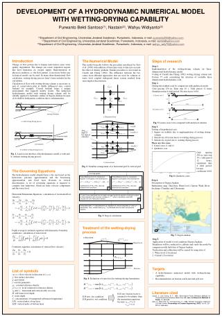
1. time step update Finite difference form of x momentum equation is arranged to the following form: Coefficients of {F1Xk, F2Xk, GXk} are obtained form calculation. Finite difference form of y momentum equation is arranged to the following form: Coefficients of {F1Yk, F2Yk, GYk} are obtained from calculation. 1 2 high tide high tide (1) and (2) are substituted into the depth averaged continuity equation resulting in system of linear equations with unknown variable of n+1, which is solved by using SOR (Successive Over Relaxation) method. minimum depth mwl mwl 3 low tide low tide moving boundary Using water level n+1 calculated from (3), equations (1) and (2) calculate ukn+1and vkn+1respectively.Then, vertical velocity wkn+1is calculated from the mass conservation equation. fix boundary 4 b) without wetting-drying process a) with wetting-drying process 0.25 m 5 m wLSX,i,j k=LSX uLSX,i,j uLSX,i+1,j CLSX,i,j 20 km i,j+1 wLSX+1,i,j SHXk,i,j = depth of flux faces at i-direction k=LSX +1 CLSX+1,i,j uLSX+1,i,j uLSX+1,i+1,j vi,j+1 i-1,j i,j, Ci,j i+1,j wLEX-1,i,j ui,j ui+1,j k=LEX -1 CLEX+1,i,j uLEX-1,i,j uLEX-1,i+1,j wLEX,i,j vi,j uLEX,i+1,j k=LEX CLEX,i,j Lokasi Studi uLEX,i,j 1.0 m i,j-1 6 m 18 km DEVELOPMENT OF A HYDRODYNAMIC NUMERICAL MODEL WITH WETTING-DRYING CAPABILITY Purwanto Bekti Santoso(1), Nastain(2), Wahyu Widiyanto(3) (1)Department of Civil Engineering, Universitas Jenderal Soedirman, Purwokerto, Indonesia, e-mail: purwanto250@yahoo.com (2)Department of Civil Engineering, Universitas Jenderal Soedirman, Purwokerto, Indonesia, e-mail: tain93@yahoo.com (3)Department of Civil Engineering, Universitas Jenderal Soedirman, Purwokerto, Indonesia, e-mail: wahyu_wdy75@yahoo.com Introduction Change of flow pattern due to human intervention cause water quality degradation. The change can create stagnation regions that have limitation on oxygen supply. Representation of physical condition, i.e. the flow pattern, is necessary before any ecological model can be used. In many three-dimensional flow calculation, wetting-drying process hasn’t been included in the calculation. Calculation of flow with wetting-drying scheme is necessary as part of conservation plan at tidally influenced area, coastal wetland for example. Coastal wetland forms a unique environment that supports nearby waters. The numerical hydrodynamic model with wetting drying scheme will be suitably applied to hydraulic studies in Segara-Anakan because of its shallow bathymetric condition due to sedimentation. The Numerical Model This model basically follows the procedure introduced by Sato et al. (1993) with addition of baroclinic term to take into account the effect of density gradient. Similar procedure is also found in Casulli and Cheng (1992). The difference between the two comes from different approaches that are used for solution of water level coupled tridiagonal linear system resulted from semi-implicit dicretization. Steps of research Step 1. Implementation of the wetting-drying scheme on three-dimensional hydrodynamic model. Coding of Casulli dan Cheng (1992) wetting drying scheme into Fortran 77 code considering the structure of available three dimensional hydrodynamic code. Step2. Testing the resulted code by comparison with analytical results Grid spacing 250 m, Time step 10 s, Tidal period 12 hours, Simulation time 4 tidal period, Friction factor 0.001 a) Linear case 1 b) Linear case 2 a) Horizontal Grid Fig. 5. Linear cases to be compared with analytical solution • Step3. • Testing of hypothetical case. • Impact on stability due to implementation of wetting drying scheme • Sensitivity of friction factorto wetting-drying process • Sensitivity of grid size to wetting-drying process • There are two cases. • Linear cases (1 and 2) • Quadratic case Grid spacing 250 m, time step 10 s, tidal period 12 hours, simulation time 4 tidal period, friction coefficient 0.001 Fig. 1. Land-ocean interface of hydrodynamics model a) with and b) without wetting-drying process b) Vertical Grid The Governing Equations The hydrodynamic model adopted here is the one based on the hydrostatic pressure approximation and the boussinesq approximation, and fixed layer divisions in vertical discretization. A set of governing equations is required to compute four unknowns, which are three velocity components and the water level. Fig. 2. Variables arrangement of a) horizontal grid b) vertical grid Fig. 6. Quadratic cases Step4. Description of Segara Anakan Bathymetric map, Tidal data, Water level, Current, Wind, River discharge(Citanduy and Cibeureum) Horizontal Momentum Equations (calculation of horizontal flow velocity) Fig. 3. Step of calculation Treatment of the wetting-drying process Depth averaged continuity equation with kinematics boundary conditions ( calculation of water level) Fig. 7. Segara anakan x-direction : Step 5. Application of model to real condition (Segara Anakan). Water level Simulation will be conductedto calibrate and verify the model by comparison with field data of Segara Anakan Continuity equation (calculation of vertical flow velocity) • Verification and calibration will be carried by using data of: • Water level (2 locations) • Current (2 locations) Targets A hydrodynamics numerical model with wetting-drying capability Recommendation on friction coefficient and grid size List of symbols (u,v,w): flow velocity in direction of (x,y,z) : free surface elevation g: gravitation f: coriolis parameter 0 : constant reference density ’(x,y,z,t): local variation to reference density h and v : horizontal and vertical eddy viscosity H: still water level depth h: water depth C: concentrations of transported substances/temperature LSX: vertical index of top layer LEX: vertical index of bottom layer Bottom Fig. 4. Definition of water level in wetting-drying formulation Literature cited Casulli, V., and Cheng, R. T., 1992. Semi-Implicit Finite Difference Methods for Three-Dimensional Shallow Water Flow, Int. Jour. for Numerical Methods in Fluids, 15, 629-648. Sato, K., Matsuoka, M., and Kazumitsu, K., 1993. Efficient calculation method of 3-D tidal current. Proceedings of Coastal Engineering, JSCE, Vol.40, 221-225.(in Japanese) If H zero friction factor is assumed to be infinite, then the momentum equations become: ui+1,jn+1= 0vi,j+1n+1= 0 If H zero, dry conditionIf H positive, wet condition