Rethinking Boundaries in Governing Equations for Ocean Modelling
460 likes | 596 Vues
This presentation explores innovative approaches to handling artificial and natural boundaries in governing equations, focusing on their effects on solutions. Addressing issues surrounding upper and lower boundary conditions, it emphasizes the importance of physical realism over analytical conformity in model setups. The choice of vertical coordinates and the implications for dynamic structures in the ocean are discussed, highlighting the trade-off between simpler equations with complex boundaries versus complex equations with simpler boundaries. Insights from observational evidence and modern coordinate transformations are presented to inspire new perspectives.

Rethinking Boundaries in Governing Equations for Ocean Modelling
E N D
Presentation Transcript
Governing Equations V by Nils Wedi (room 007; ext. 2657) Thanks to Piotr Smolarkiewicz and Peter Bechtold
Introduction and motivation • How do we treat artificial and/or natural boundaries and how do these influence the solution ? • Highlight issues with respect to upper and lower boundary conditions. • Inspire a different thinking with respect to boundaries, which are an integral part of the equations and their respective solution.
Observations of boundary layers: the tropical thermocline M. Balmaseda
Observations of boundary layers: EPIC - PBL over oceans M. Koehler
Boundaries • We are used to assuming a particular boundary that fits the analytical or numerical framework but not necessarily physical free surface, non-reflecting boundary, etc. • Often the chosen numerical framework (and in particular the choice of the vertical coordinate in global models) favours a particular boundary condition where its influence on the solution remains unclear. • Horizontal boundaries in limited-area models often cause excessive rainfall at the edges and are an ongoing subject of research (often some form of gradual nesting of different model resolutions applied).
Choice of vertical coordinate • Ocean modellers claim that only isopycnic/isentropic frameworks maintain dynamic structures over many (life-)cycles ? … Because coordinates are not subject to truncation errors in ordinary frameworks. • There is a believe that terrain following coordinate transformations are problematic in higher resolution due to apparent effects of error spreading into regions far away from the boundary in particular PV distortion. However, in most cases problems could be traced back to implementation issues which are more demanding and possibly less robust to alterations. • Note, that in higher resolutions the PV concept may loose some of its virtues since the fields are not smooth anymore, and isentropes steepen and overturn.
Choice of vertical coordinate • Hybridization or layering to exploit the strength of various coordinates in different regions (in particular boundary regions) of the model domain • Unstructured meshes: CFD applications typically model only simple fluids in complex geometry, in contrast atmospheric flows are complicated fluid flows in relatively simple geometry (eg. gravity wave breaking at high altitude, trapped waves, shear flows etc.) Bacon et al. (2000)
But why making the equations more difficult ? • Choice 1: Use relatively simple equations with difficult boundaries or • Choice 2: Use complicated equations with simple boundaries • The latter exploits the beauty of “A metric structure determined by data” Freudenthal, Dictionary of Scientific Biography (Riemann), C.C. Gillispie, Scribner & Sons New York (1970-1980)
Examples of vertical boundary simplifications • Radiative boundaries can also be difficult to implement, simple is perhaps relative • Absorbing layers are easy to implement but their effect has to be evaluated/tuned for each problem at hand • For some choices of prognostic variables (such as in the nonhydrostatic version of IFS) there are particular difficulties with ‘absorbing layers’
Radiative Boundary Conditions for limited height models eg.Klemp and Durran (1983); Bougeault (1983); Givoli (1991); Herzog (1995); Durran (1999) Linearized Boussinesq Equations in x-z plane
Radiative Boundary Conditions Inserting… Dispersion relation: Phase speed: for hydrostatic waves Group velocity:
Radiative Boundary Conditions discretized Fourier series coefficients:
Wave-absorbing layers eg. Durran (1999) Adding r.h.s. terms of the form … Viscous damping: Rayleigh damping: Note, that a similar term in the thermodynamic equation mimics radiative damping and is also called Newtonian cooling.
Flow past Scandinavia 60h forecast 17/03/1998 horizontal divergence patterns in the operational configuration
Flow past Scandinavia 60h forecast 17/03/1998horizontal divergence patterns with no absorbers aloft
Wave-absorbing layers: overlapping absorber regions Finite difference example of an implicit absorber treatment including overlapping regions
The second choice … • Observational evidence of time-dependent well-marked surfaces, characterized by strong vertical gradients, ‘interfacing’ stratified flows with well-mixed layers Can we use the knowledge of the time evolution of the interface ?
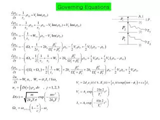
Generalized coordinate equations Strong conservation formulation !
Explanations … Using: Jacobian of the transformation Transformation coefficients Contravariant velocity Solenoidal velocity Physical velocity
Time-dependent curvilinear boundaries • Extending Gal-Chen and Somerville terrain-following coordinate transformation on time-dependent curvilinear boundaries Wedi and Smolarkiewicz (2004)
Swinging membrane Animation: Swinging membranes bounding a homogeneous Boussinesq fluid
Another practical example • Incorporate an approximate free-surface boundary into non-hydrostatic ocean models • “Single layer” simulation with an auxiliary boundary model given by the solution of the shallow water equations • Comparison to a “two-layer” simulation with density discontinuity 1/1000
supercritical Critical, downstream propagating lee jump critical, stationary lee jump subcritical Regime diagram
Critical – reduced domain flat shallow water
Numerical modelling of the quasi-biennial oscillation (QBO) analogue • An example of a zonal mean zonal flow entirely driven by the oscillation of a boundary!
The laboratory experiment of Plumb and McEwan • The principal mechanism of the QBO was demonstrated in the laboratory • University of Kyoto Plumb and McEwan, J. Atmos. Sci. 35 1827-1839 (1978) http://www.gfd-dennou.org/library/gfd_exp/exp_e/index.htm Animation: Note: In the laboratory there is only molecular viscosity and the diffusivity of salt. In the atmosphere there is also radiative damping.
Time dependent boundaries Wedi and Smolarkiewicz, J. Comput. Phys 193(1) (2004) 1-20 Time-dependent coordinate transformation
Time – height cross section of the mean flow Uin a 3D simulation Animation (Wedi and Smolarkiewicz, J. Atmos. Sci., 2006)
Waves propagating right Waves propagating right +U wave interference Critical layer progresses downward S = 8 U U filtering filtering (b) (a) Waves propagating left Waves propagating left U wave interference Critical layer progresses downward S = +8 +U +U filtering filtering (c) (d) Schematic description of the QBO laboratory analogue
The stratospheric QBO • westward • + eastward (unfiltered) ERA40 data (Uppala et al, 2005)
Stratospheric mean flow oscillations • In the laboratory the gravity waves generated by the oscillating boundary and their interaction are the primary reason for the mean flow oscillation. • In the stratosphere there are numerous gravity wave sources which in concert produce the stratospheric mean flow oscillations such as QBO and SAO (semi-annual oscillation).
Numerically generated forcing! Instantaneous horizontal velocity divergence at ~100hPa No convection parameterization Tiedke massflux scheme T63 L91 IFS simulation over 4 years
Modelling the QBO in IFS ? • Not really, due to the lack of vertical resolution to resolve dissipation processes of gravity waves, possibly also due the lack of appropriate stratospheric radiative damping, but certainly due to the lack of sufficient vertically propagating gravity wave sources, which may in part be from convection, which in itsself is a parameterized process. • A solution is to incorporate (parameterized) sources of (non-orographic) gravity waves. These parameterization schemes incorporate the sources, propagation and dissipation of momentum carried by the gravity waves into the upper atmosphere (typically < 100hPa) • The QBO is perhaps of less importance in NWP but vertically propagating waves (either artificially generated or resolved) and their influence on the mean global circulation are very important!
July climatology SPARC 35r2
July climatology SPARC 35r3
QBO : Hovmöller from free 6y integrations =no nonoro GWD Difficult to find the right level of tuning !!!
Parametrized non-orographic gravity wave momentum flux Comparison of observed and parametrized GW momentum flux for 8-14 August 1997 horizontal distributions of absolute values of momentum flux (mPa) Observed values are for CRISTA-2 (Ern et al. 2006). Observations measure temperature fluctuations with infrared spectrometer, momentum fluxes are derived via conversion formula.
Total = resolved + parametrized wave momentum flux A. Orr, P. Bechtold, J. Scinoccia, M. Ern, M. Janiskova (JAS 2009 to be submitted)
Resolved and unresolved gravity waves • The impact of resolved and unresolved gravity waves on the circulation and model bias remains an active area of research. • Note the apparent conflict of designing robust and efficient numerical methods (i.e. implicit methods aiming to artificially reduce the propagation speed of vertically propagating gravity waves or even the filtering of gravity waves such as to allow the use of large time-steps) and the important influence of precisely those gravity waves on the overall circulation. Most likely, the same conflict does not exist with respect to acoustic waves, however, making their a-priori filtering feasible.