Remote Sensing of the Oceans

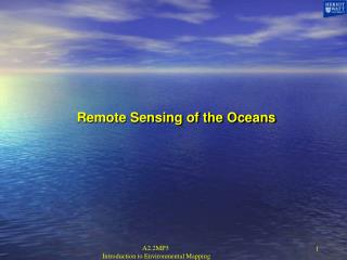
1. Remote Sensing of the Oceans A2.2MP3 Introduction to Environmental Mapping

2. Key Issues • Large scale dynamical patterns in the oceans • Surface water temperature and evidence of changes • Distribution of sea ice and year-on-year changes • Biological productivity • Topography and composition of the seabed A2.2MP3 Introduction to Environmental Mapping

3. Contents • Satellites used • Topography of the sea surface • Sea surface temperatures • Surface currents and water masses • Sea ice • Ocean colour • Marine Animal Tracking A2.2MP3 Introduction to Environmental Mapping

4. Satellites and Instruments

5. Why Remote Sensing? • Perhaps more than any other area of the planet surface satellite remote sensing provides a means of widespread and repetitive measurements of the oceans. • Man has been investigating the worlds oceans for over 300 years. All of our understanding has come from “point” measurements. That is sampling taken by scientists on a vessel at a particular spot (and for a short time interval) on the ocean surface. • Because of this it was very difficult to interrelate phenomenon occurring over large geographic areas or at different time of the year. • This is an area in which Satellite sensing excels! A2.2MP3 Introduction to Environmental Mapping

6. The Advance Very High resolution Radiometer (NOAA) • This is one of the most widely used oceanographic monitoring satellites. The scanner collects information in five bands which include the visible, near-infrared, and thermal infrared portions of the electromagnetic spectrum. • AVHRR data are acquired in three formats: High Resolution Picture Transmission (HRPT) images are transmitted to a ground station in real-time. Local Area Coverage (LAC) data are the same images recorded on tape for later transmission. Global Area Coverage (GAC) represents imagery that is resampled to 4 km. • Spatial Resolution: 1.1 km (LAC and HRPT) and 4 km (GAC) • Temporal Resolution: twice/day • Spectral Resolution: Band 1 2 3 4 5 Wavelength (mm) .58 to .68, .725 to 1.10, 3.55 to 3.93, 10.3 to 11.3, 11.5 to 12.5 • Orbit: near polar, sun-synchronous, 833 km in altitude • Swath Width : 2399 km A2.2MP3 Introduction to Environmental Mapping

7. SeaWiFS (NASA) • The Sea-viewing Wide-Field-of View Sensor on board the SeaStar spacecraft is an advanced sensor designed for ocean monitoring, specifically the observation of ocean color. The SeaWiFS sensor consists of eight spectral bands of very narrow wavelength ranges tailored for very specific detection and monitoring of various ocean phenomena including ocean primary production and phytoplankton processes. These applications require calibration with in situ data. • Data is available in three formats: High Resolution Picture Transmission (HRPT), which is real-time data and Local Area Coverage (LAC), which is recorded data, have a spatial resolution of .88 km and swath width of 2800 km. Global Area Coverage (GAC), has a spatial resolution of 4 km and a swath width of 1500 km. • Dates of Operation: 9/18/97 to present • Spatial Resolution: 0.88 km (LAC and HRPT) and 4 km (GAC) (scanner can be tilted 20 degrees from nadir in either direction) • Temporal Resolution: 1 visit/day • Spectral Resolution Band 1 2 3 4 5 Wavelength (mm) .58 to .68, .725 to 1.10, 3.55 to 3.93, 10.3 to 11.3 ,11.5 to 12.5 • Orbit: near-polar, sun-synchronous, 705 km in altitude A2.2MP3 Introduction to Environmental Mapping

8. Coastal Zone Colour Scanner (NASA) • The Coastal Zone Colour Scanner was launched in 1978 with the goal of monitoring the Earth’s oceans and water bodies. Its main objective was to observe ocean colour and temperature, particularly in the coastal zone. It was the first instrument with sufficient spatial and spectral resolution to detect pollutants in the upper levels of the ocean and to distinguish suspended materials in the water column. CZCS was eventually replaced by SeaWiFS. • Dates of Operation: November, 1978 to June, 1986 on board Nimbus-7 • Spatial Resolution: 825 m • Temporal Resolution: daily • Spectral Resolution: Band 1 2 3 4 5 6* Wavelength (mm) .43 - .45, .51 - .53, .54 - .56, .66 - .68, .70 - .80, 10.5 - 12.50 *not functional beyond 1979 • Radiometric Resolution: 8 bit • Orbit: near-polar, sun-synchronous, at an altitude of 955 km • Swath Width: 1566 km • Applications: ocean color, pigment concentrations, sediment distribution A2.2MP3 Introduction to Environmental Mapping

9. RADARSAT • RADARSAT is a relatively recent spaceborne SAR system, launched on November 4, 1995. RADARSAT is managed by the Canadian Space Agency. It is a highly flexible sensor capable of a variety of imaging configurations and applications. • Dates of Operation: 11/4/95 to present • Modes of Operation: RADARSAT is an extremely versatile instrument with seven modes of operation and multiple beam positions within those modes. • Temporal Resolution: revisit every 24 days, with 7- and 3-day revisit times possible. • Orbit: near-polar, sun synchronous with an altitude of 798 km • Applications : ocean features; coastal zone mapping; ship detection; oil spill detection A2.2MP3 Introduction to Environmental Mapping

10. Radarsat SAR Operations A2.2MP3 Introduction to Environmental Mapping

11. TOPEX/POSIEDON (http://www.tsgc.utexas.edu/topex/activities/topex_basics/index.html) • Launched in August of 1992, the T/P satellite has mapped ocean surface topography for over 95% of the world's ice-free seas. • It does this by making very precise and accurate measurements of sea surface height. A2.2MP3 Introduction to Environmental Mapping

12. The satellite passes over the same ground spot once every 10 days. T/P's ground tracks cover over 95% of the ice-free oceans every 10 days. During its first month of operation, T/P collected more ocean data than all the ships had for the past 100 years! • T/P has 2 altimeters that measure the distance from the satellite to the ocean. These altimeters send radar signals straight down which "bounce off" the ocean surface. The time it takes for the radar signal to return to the satellite tells us how far the satellite is from the ocean's surface. A2.2MP3 Introduction to Environmental Mapping

13. A2.2MP3 Introduction to Environmental Mapping

14. Sea Surface Physical Properties Height (deviation from “average”) Waves Wind Currents

15. The Importance of these Parameters • Oceanographic science/ understanding • Understanding of climate change/ weather • Hurricane and Typhoon notification • Ship routing • Oil and gas operations A2.2MP3 Introduction to Environmental Mapping

16. Surface Height • The topography of the sea surface can be measured accurately using radar altimetry. • The differences in level arise from thermal heating of the ocean surface, combined with the effect of the Coriolis force due to the Earth’s rotation. • Long term changes may reflect melting of the polar ice caps. • The relative levels of the ocean surface provide a pressure difference that drives the surface current system of the oceans. • Thus a map of the dynamic height of the ocean is equivalent to a meteorological pressure chart and can be interpreted in a similar way A2.2MP3 Introduction to Environmental Mapping

17. Properties that can be measured • Surface “height”. The time taken for the radar pulse to travel to the water surface and back to the satellite can be used to measure the deflection of the water surface. • The shape of the returned pulse can be used to measure • Wave height • Surface currents • Temperature • Wind speed can be inferred from the signal due to surface “ripples” A2.2MP3 Introduction to Environmental Mapping

18. Mean Sea-Surface Topography A2.2MP3 Introduction to Environmental Mapping

19. Wind Speeds and Wave heights3-12 October 1992 – Topex Poseidon A2.2MP3 Introduction to Environmental Mapping

20. Ocean Winds • QuikScat will provide climatologists, meteorologists and oceanographers with daily, detailed snapshots of the winds swirling above the world's oceans. Pacific Surface Winds - This animation shows ocean surface wind speeds and directions over the Pacific as measured by the NSCAT scatterometer on September 20, 1996 A2.2MP3 Introduction to Environmental Mapping

21. Wind Currents in the Pacific A2.2MP3 Introduction to Environmental Mapping

22. Sea surface temperatures

23. Sea surface temperatures (SST) are routinely measured by the AVHRR instrument on the NOAA weather satellites, as well as by more specialised instruments such as those on SeaStar. • SSTs allow us to visualise: • the global distribution of temperature • local and regional currents and water masses (due to temperature differences between different water masses). • the development of events such as El Niño. • Long term measurements of SST are important in the calibration of global climate models and in monitoring global climatic change. A2.2MP3 Introduction to Environmental Mapping

24. Mean annual sea surface temperature A2.2MP3 Introduction to Environmental Mapping

25. Sea surface temperature A2.2MP3 Introduction to Environmental Mapping

26. Gulf stream – thermal and example of a permanent temperature difference A2.2MP3 Introduction to Environmental Mapping

27. Ocean colour

28. ‘Ocean colour’ is the name given to the false colour images obtained from different reflectances at closely spaced bands within the optical and near infrared spectrum. • These reflectances arise from specific algal pigments in the water column and are a measure of biogenic productivity. This is entirely analogous to the discussion regards vegetative material on land. A2.2MP3 Introduction to Environmental Mapping

29. Phytoplankton • Phytoplankton are the first link in the marine food web • Just like plants on land, phytoplankton require light, water, carbon dioxide and nutrients to grow (photosynthesis) • The observed patterns of distribution of phytoplankton are related to physical and biological processes • They play a key role in the ecology of the marine ecosystem and changes in their patterns of distribution and abundance can have significant impact on the entire ecosystem • Phytoplankton have a major role in the global carbon cycle (50% of the Earths photosynthesis is through phytoplankton – but 90% of the Earths CO2 is now in marine sediments) • They can be dangerous (Algal bloom and toxicity). A2.2MP3 Introduction to Environmental Mapping

30. The original ocean colour investigations were carried out by the experimental coastal zone color scanner (CZCS) on the Nimbus-7 satellite. • These studies are now continued on a routine basis by the SeaWiFS instrument carried on the SeaStar satellite. • SeaWiFS is an eight channel multispectral scanner operating in the optical band between 400-800 nm. Two resolutions are used: Local area (1km) and Global (4km), with a swath width for both of 2800km. A2.2MP3 Introduction to Environmental Mapping

31. Spectral bands of the Nimbus CZCS 430-450 nm Chlorophyll absorption (green) 510-530 nm Chlorophyll concentration (green) 560-580 nm Gelbostoffe (yellow) 660-680 nm Aerosol absorption (red) 700-800 nm Surface vegetation (near IR) 1050-1250 nm Surface temperature (Thermal IR) A2.2MP3 Introduction to Environmental Mapping

32. Ocean colour is a measure of nutrient availability. • It varies with water temperature, geographical setting and with the season. • Strong ocean colour arises when nutrients are readily available. Example settings include: • Upwelling of deeper, colder water at ocean margins • Full-depth mixing in shallow seas and bays • Local input from terrestrial sources such as rivers • Turbulent interaction of water masses at oceanic fronts A2.2MP3 Introduction to Environmental Mapping

33. THE NDVI IS USED AS A MEASURE OF CHLOROPHYLL ABUNDANCE IN THE SAME WAY AS BEFORE. A2.2MP3 Introduction to Environmental Mapping

34. Some Examples A2.2MP3 Introduction to Environmental Mapping

35. The North Atlantic Bloom A2.2MP3 Introduction to Environmental Mapping

36. Ocean Circulation Patterns A2.2MP3 Introduction to Environmental Mapping

37. Example: El Nino • Under normal circumstances there is a strong “upswelling” of cool waters in the equatorial regions to the west of the South American coast. A2.2MP3 Introduction to Environmental Mapping

38. Effects of Current and Upswelling • This upswelling brings nutrient rich waters to the surface. Phytoplankton and hence fish etc. depend on the nutrient brought up by the current • El Nino (The Boy Child) is the name for the suppression of this strong upswelling by a warmer surface current. Sea temperatures can be several degrees higher than normal • This has considerable consequence for • Distribution of phytoplankton and hence fish • Weather systems (local and global) A2.2MP3 Introduction to Environmental Mapping

39. The El Nino Condition A2.2MP3 Introduction to Environmental Mapping

40. Impact on Marine Life • At Christmas Island, as a result of the sea level rise during the 1982-83 El Niño, sea birds abandoned their young and flew out over a wide expanse of ocean in a desperate search for food. Along the coast of Peru during that same time period, 25 percent of the adult fur seal and sea lion populations starved to death, and all of the pups in both populations died. Similar losses were experienced in many fish populations. • The 1982-83 El Niño is estimated by NOAA to have caused some $8 billion in damages due to floods, severe storms, droughts and fires around the world. A2.2MP3 Introduction to Environmental Mapping

41. El Niño's impacts on weather patterns • El Niño's effects are not limited to the tropical regions off the western coasts of Peru and Ecuador. Its effects are felt all over the world, where the disruption of normal local weather patterns can have tragic and/or profound economic consequences. Increased heat and moisture rises into the atmosphere, altering the weather patterns in neighboring regions, which can ripple out to affect other region weather patterns around the globe. For instance, a severe El Niño will enhance the jet stream over the western Pacific and shift it eastward, leading to stronger winter storms over California and the southern United States, with accompanying floods and landslides. In contrast, El Niño can also cause severe droughts over Australia, Indonesia, and parts of southern Asia. A2.2MP3 Introduction to Environmental Mapping

42. El Nino – Temperature Variations El Nino Event Normal Conditions A2.2MP3 Introduction to Environmental Mapping

43. “El Nino” Effect on Phytoplankton El- Nino Event September to November 1997 Normal Condition June to August 1998 A2.2MP3 Introduction to Environmental Mapping

44. Remember animation A2.2MP3 Introduction to Environmental Mapping

45. The Effect of Nutrient Input from a River Nutrient input from the Orinoco river A2.2MP3 Introduction to Environmental Mapping

46. The Effect of Weather Conditions Effect of monsoonal circulation - southerly winds Effect of monsoonal circulation - northerly winds A2.2MP3 Introduction to Environmental Mapping

47. Algal Bloom in the Bering Sea • The massive bloom of in the Bering Sea of the coccolithophores has never before been observed there. • They may be another sign of a larger transformation in the surrounding ecosystem. • The bloom's presence coincides with lower salmon counts along the coasts, a redistribution of microscopic animals in the surrounding ocean, and the massive deaths of shearwaters–hook billed, surface-feeding seabirds related to the albatross. • These events may spell major trouble for the Bering Sea ecosystem and the fisheries that ply these waters. A2.2MP3 Introduction to Environmental Mapping

48. True colour image (a detail of the April 25, 1998 image) from the SeaWiFS instrument shows the bright reflection caused by billions of coccoliths. Alaska and the Bering Sea from SeaWiFS on April 25, 1998. The bright aquamarine water is caused by the huge numbers of coccolithophores. A2.2MP3 Introduction to Environmental Mapping

49. After a Reduction This satellite image of the Bering Sea was acquired on July 20, 1998. The mottled water just off the coast of Alaska remains relatively free of coccolithophores—instead it is coloured brown by silt. A2.2MP3 Introduction to Environmental Mapping

50. The global surface circulation and Phytoplankton Distribution A2.2MP3 Introduction to Environmental Mapping