
Research Presentation: Overview of Work Done in 2006
E N D
Presentation Transcript
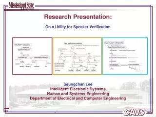
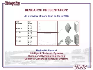
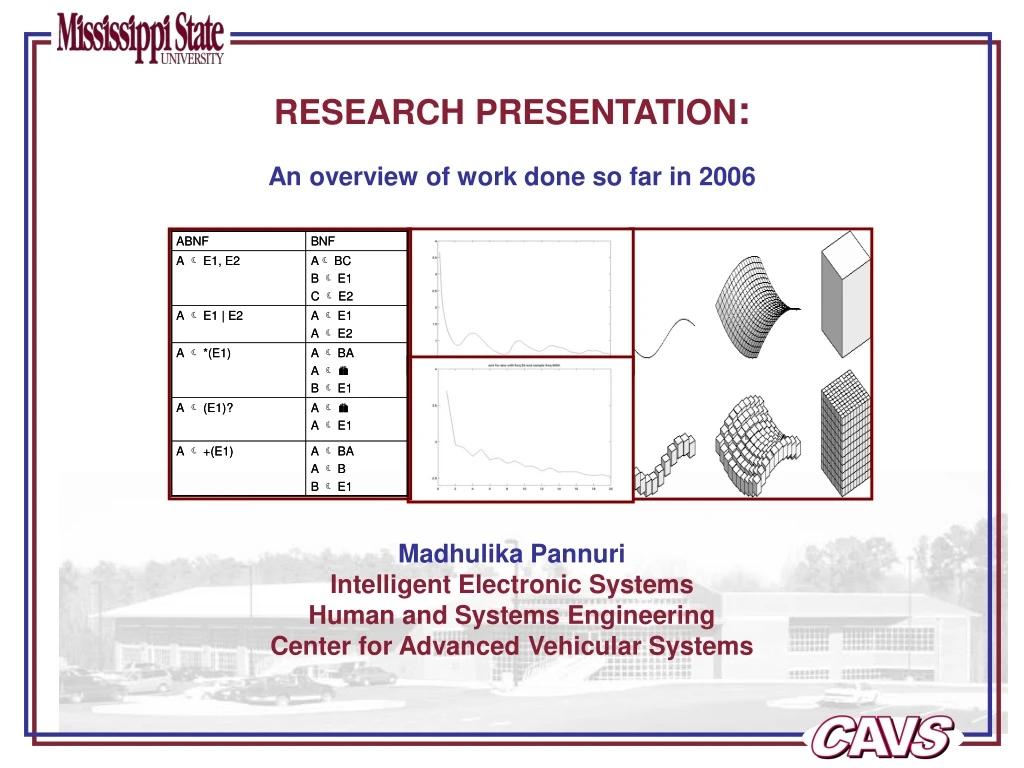
RESEARCH PRESENTATION: An overview of work done so far in 2006 Madhulika Pannuri Intelligent Electronic Systems Human and Systems Engineering Center for Advanced Vehicular Systems
Abstract • Language Model ABNF: • The LanguageModel ABNF reads in a set of productions in the form of ABNF and converts them to BNF. These productions are passed to LanguageModel BNF in the form they were received. • Optimum time Delay estimation: • Computes optimum time delay for re-constructing phase space. Auto Mutual Information is used for finding optimum time delay. • Dimension Estimation: • The dimension of an attractor is a measure of its geometric scaling properties and is ‘the most basic property of an attractor’. Though there are many dimensions, we will be implementing ‘Correlation Dimension’ and ‘Lyapunov Dimension’.
Language Model ABNF • Why conversion from ABNF to BNF? • ABNF balances compactness and simplicity, with reasonable representational power. • Differences: The differences between BNF and ABNF involve naming rules, repetition, alternatives, order-independence and value ranges. • Removing the meta symbols makes it easy to convert it to finite state machines (IHD). • Problem: Converting any given ABNF production to BNF is impossible. So, generalize the algorithm so that most of the expressions can be converted. • The steps for conversion involve removing meta symbols one after the other. There were complications like multiple nesting. • Ex: * (+(a, n) | (b | s))
Language Model ABNF • Concatenation: • Removing concatenation requires two new rules with new names to be introduced. The last two productions resulting from conversion are not valid CFG’s but shorter than the original. • Alternation: • The production is replaced with a pair of productions. They may or may not be legal CFG’s. • Kleene Star: • New variable is introduced and the production is replaced. Gives rise to epsilon transition. • Kleene Plus: • Similar to Kleene Plus. No null transition.
Optimum time delay estimation • Why calculating time delay ? • If we have a trajectory from a chaotic system and we only have data from one of the system variables, there's a neat theorem that says that a copy of the attractor of the system can be reconstructed by lagging the time series to embed it in more dimensions. • In other words, if we have a point F( x, y, z, t) which is along some strange attractor, and we can only measure F(z,t), we can plot F (z, z + N, z + 2N, t), and the resulting object will be topologically identical to the original attractor ..!!! • Method of time delays provides a relatively simple way of constructing an attractor from single experimental time series. • Can I choose some value randomly ?? • NO. Choosing optimum time delay is not trivial as the dynamical properties of the reconstructed attractor are to be amenable for subsequent analysis. • For an infinite amount of noise free data, we are free to choose arbitrarily, the time delay.
Optimum time delay estimation • For smaller values of tau, s(t) and s(t+tau) are very close to each other in numerical value, and hence they are not independent of each other. • For large values of tau, s(t) and s(t+ tau) are completely independent of each other, and any connection between them in the case of chaotic attractor is random because of butterfly effect. • We need a criterion for intermediate choice that is large enough so that s(t) and s(t+tau) are independent but not so large that s(t) and s(t+tau) are completely independent in statistical sense. • Time delay is a multiple of sampling time (data is available at these times only). • There are four common methods for determining an optimum time delay: • Visual Inspection of reconstructed attractors: • The simplest way to choose tau. • Consider successively larger values of tau and then visually inspect the phase portrait of the resulting attractor. • Choose the tau value which appears to give the most spread out attractor. • Disadvantage: • This produces reasonable results with simple systems only.
Methods to estimate optimum time delay • 2. Dominant period relationship: • We use the property that time delay is one quarter of the dominant period. • Advantage: • Quick and easy method for determining tau. • Disadvantages: • Can be used for low dimensional systems only. • Many complex systems do not possess a single dominant frequency. • The Autocorrelation function: • The auto correlation function rk, compares two data points in the time series separated by delay k, and is defined as, • The delay for the attractor reconstruction, tau, is then taken at a specific threshold The behavior of correlation is inconsistent .
Mutual Information Method • 4.Minimum auto mutual Information method: • The Mutual Information is given by: • When the mutual information is minimum, the attractor is as spread out as much as possible. This condition for the choice of delay time is known as ‘minimum mutual informationcriterion’. • Practical Implementation: • To calculate the mutual information, the 2D reconstruction of an attractor is partitioned into a grid of Nc columns and Nr rows. • Discrete probability density functions for X(i) and X(i+tau) are generated by summing the data points in each row and column of the grid respectively and dividing by the total number of attractor points. • The joint probability of occurrence P(k, l) of the attractor in any particular box is calculated by counting the number of discrete points in the box and dividing by the total number of points on the attractor trajectory. • The value of tau which gives the first minimum is the attractor reconstruction delay.
ami vs auto correlation • Mutual information is a function of both linear and non linear dependencies between two variables. Where as correlation is function of linear dependencies only. • The plots below show mutual information and correlation for Lorenz time series. • As seen correlation function has a mean at tau ~ 30 and mutual information has a first minimum at tau ~ 12. • Which one do I consider ?? • The answer can be found simply by plotting reconstructed phase space with both the tau values and compare with the actual attractor.
Reconstructed phase space (Lorenz) • Two plots below show reconstructed phase space for tau value 15 ( in the case of ami) and 30 ( as shown by correlation). • http://www.cavs.msstate.edu/~pannuri/lorenz.recon.anim.0-50.gif • As can be seen from the plots below, the attractor looks clean and opened up at tau = 15. At tau = 30, the attractor is quite unrecognizable.
Dimension Estimation (Next task) • Many definitions of dimension exist. Out of all, we are interested in four types. • Though we will not be implementing all the four, it would be nice to know them. • 1. Box Counting Dimension or Capacity Dimension: • Simple and easily understood of all.
Dimension estimation (next task) • The Information Dimension: • Instead of simply counting each cube which contains part of attractor, how much of the attractor is contained within each cube is calculated. • This measure seeks the differences in the distribution density points covering the attractor. • For the case with evenly distributed points, information dimension is same as box counting dimension. • Correlation Dimension: • Why correlation dimension ? • Calculating box counting dimension and information dimension require a prohibitive amount of computation time. • The correlation dimension may be defined as follows: • More formally correlation dimension is defined using Heaviside function:
Correlation Dimension • The hyper sphere is constructed with one of the points as center. • The number of points on the attractor with in the hypersphere are counted. (Heaviside function does this) • The Heaviside function is equal to unity if the distance between two points is less than hyper sphere radius; otherwise value zero is returned. • The calculation of correlation sum involves following the reference trajectory, stopping at each discrete point and counting the number of attractor points within the hypersphere. • The cumulative sum is then divided by N(N – 1) to get the correlation dimension. • The maximum value of correlation dimension is 1 and is attained when radius of the probing hypersphere is greater than the attractor’s largest diameter and all the points are counted
Dimension estimation • Lyapunov Dimension: • Relationship between fractal dimension and their spectrum of Lyapunov exponents. • The most useful of all the dimensions. • Based on dynamics rather than on geometry. • Defined in terms of Lyapunov exponents (which describe the dynamics of a system). • The Lyapunov dimension may be defines as:
Next Tasks • These are the assignments I will be working on rest of month. • Task 1: • Applying mutual information and finding tau for various phones ( on speech ). • Task 2: • Finding the correlation dimension and testing it for various time series. • Task 3: • Finding Lyapunov dimension.
Summary • Langauage Model ABNF removes the complexities in ABNF by removing meta symbols. • Mutual Information estimation is the best method to estimate optimum time delay. • The invariance of the tau value with variation in the parameters like the number of bins makes it better than correlation. • Lyapunov dimension and Correlation dimension are the most useful dimensions.
References • Language Model ABNF: • Java Speech Grammar Format Specification, Version 1, Sun Microsystems Developer Network, October 26, 1998 (see http://java.sun.com/products/java/media/speech/forDevelopers/JSGF/JSGF). • A. Hunt and S. McGlashan, Eds., W3C Speech Recognition Grammar Specification Version 1.0, March 16, 2004 (see http://www.w3.org/TR/speech-grammar/). • J. Picone, et al., “A Public Domain C++ Speech Recognition Toolkit,” Center for Advanced Vehicular Systems, Mississippi State University, Mississippi State, MS, USA, January 2006. • J.E. Hopcroft, R. Motwani and J. D. Ullman, Introduction to Automata Theory, Languages, and Computation, Addison Wesley, Boston, MA, 2001. • D. Jurafsky and J. H. Martin, Speech and Language Processing, Pearson, Singapore, 2000 • Optimum time delay estimation and dimension estimation: • P. S. Addison, Fractals and chaos, Institute of Physics publishing, London, U.K.,1997. • H. Kantz and T. Schreiber, Nonlinear Time Series Analysis, Second Edition, Cambridge University Press , U.K., 2004. • A. H. Nayfeh, B. Balachandran, Applied Nonlinear Dynamics, Wiley-Interscience Publication, NewYork, USA, 1995.