Coupled Physical/Bio-Optical Model Experiments at LEO-15

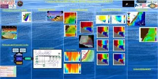
1. Coupled Physical/Bio-Optical Model Experiments at LEO-15 National Undersea Research Program Air/Sea CO2 Dust Physical Mixing and Advection Light Iron CO2 NH4 NO3 PO4 SiO4 Relict DOM Coastal Diatoms Pelagic Diatoms Dino- flagellate Synecho- coccus Excreted DOM Lysed DOM Hetero- Flagellet Viruses Copepod Ciliates LEO Bacteria Sediment Detritus Predator Closure A-Line Operational Low-Res COAMPS ATM Model Experimental High-Res COAMPS ATM Model ATM Coupler ROMS Ocean Model EcoSim Bio-Optical Model Bottom Boundary Layer Model Hernan G. Arango, Paul Bissett, Scott M. Glenn, Oscar Schofield Institute of Marine and Coastal Sciences, Rutgers University, New Brunswick, N.J. Bio-Optical Model Downwelling Event Bio-Optical Forecasts Conclusions Atmosphere-Ocean Models Ocean color is a function of the mass of optical constituents in the water column, the inherent optical properties of those constituents, and the apparent illumination of the ocean. One of the goals of ONR’s Environmental Optics Hyperspectral Coastal Ocean Dynamics Experiment (HyCODE) program is to develop the forecasting ability to predict the depth-dependent optical constituents and their impact on water-leaving radiance. One of the most intense events during the coastal predictive skill experiment occurred in forecast cycle 3, July 18-20. Strong NE winds from a Northeastern resulted in a very intense downwelling event along the New Jersey Coast. Figure 7 shows the high resolution COAMPS forecast for July 20, 12:30 with surface winds ranging between 25-30 m/s. The ocean response is immediate, as illustrated in ROMS forecast (Figures 8-10). Figures 16-22 show seleted EcoSim predicted ecological fields for July 20 along the A-line section. These figures focus on the distribution of pigmented biomass in response to the strong downwelling event between July 18-20. The fourth and final Coastal Predictive Skill Experiment (CPSE) at the Rutgers University Longterm Ecosystem Observatory (LEO) was conducted from July 11 through August 7, 2001. Ensembles of atmosphere and ocean forecasts were generated twice per week for four consecutive weeks. The Navy Operational Global Atmospheric Prediction System (NOGAPS), and the atmospheric component of the Coupled Ocean Atmospheric Mesoscale Prediction System (COAMPS) was used to drive the Regional Ocean Modeling System (ROMS) to generate real-time forecasts of 3D circulation in the Mid-Atlantic Bight (Figure 1). These ocean forecasts were used to Unfortunately, strong storm conditions usually mean limited remote sensing data. The sky cleared by the 21st and showed the impacts of the downwelling conditions that drove the warm, biomass rich waters in towards the shore (Figure 22). This can be seen as well in the predictions of chlorophyll as well (Figure 23). Figure 5: Depth dependent optical constituents. Figure 1: Ocean Model bathymetry. In pursuit of this goal, a previously developed ecological model (Ecological Simulation, EcoSim) that incorporated the Inherent and Apparent Optical Properties (IOPs and AOPs) of the water-column as a means of developing niche separation between phytoplankton species in open ocean environments was expanded and improved for coastal ocean applications. The EcoSim model that is coupled to the ROMS model in the New Jersey Bight includes 4 functional groups of phytoplankton that each includes stocks of Particulate Organic Carbon (POC), Particulate Organic Nitrogen (PON), Particulate Organic Phosphorus (POP), and Particulate Organic Iron (POFe), and for diatom groups, Particulate Organic Silica (POS). These particulate ratios of carbon, nitrogen, phosphorus, iron, and silica are allowed to vary in non-stoichiometric proportions to consider the impacts of non-“Redfield” dynamics in both inorganic and organic nutrient acquisition and growth. Each phytoplankton species has a unique set of photosynthetic and photoprotective pigments that are allowed to vary as a function of light and nutrient history. These pigments, when coupled to the hyperspectral scalar irradiance light field allow for the direct calculation of photosynthetic efficiency and photon utilization in the calculation of light dependent growth.   The model also includes 2 classes each of Colored Dissolved Organic Matter (CDOM), Dissolved Organic Carbon (DOC), Dissolved Organic Nitrogen (DON), and Dissolved Organic Phosphorus (DOP). Bacteria in the form of carbon, nitrogen, and phosphorus (BC, BN, BP, respectively) are included as remineralizers of the organic nutrient pools. The fecal forms of carbon, nitrogen, phosphorus, iron, and silica, (FC, FN, FP, FF, and FS, respectively) are included as well. Lastly, stocks of carbon, nitrate, ammonium, phosphorus, iron, and silica serve as inorganic nutrient stocks. The total number of ecological tracers for this version of EcoSim is 61. Figure 7: MSL pressure and winds at 10 m. Figure 14: A-line temperature observations. Figure 15: Observed Chlorophyll Fluorescence. The various data gathered by the observational network at the Long-Term Ecosystem Observatory (LEO-15) is used to initialize, update, and validate the coastal prediction system. These included: satellite derived sea surface temperature, CODAR-derived surface currents, CTD data from an undulating shipboard tow-body, and an autonomous underwater Glider. Ocean forecasts from each ROMS ensemble were evaluated in real-time using ADCP and remotely-profiled CTD data from the LEO underwater nodes Figure 22: SeaWiFS Observed Chlorophyll a. While the predictions appear to resolve general features, the total quantity of biomass appears to be lower than in the satellite-derived estimates. This discrepancy appears in other satellite/prediction comparisons, as well as cross-sections from other days. This appears to result in part from an over-estimation of the biomass loss from grazing and mortality. Figure 9: A-line temperature cross-section. Figure 8: Temperature and currents at –2 m. Figure 16: Total Chlorophyll-a (g/liter). Figure 17: Large diatoms Chlorphyll-a (g/liter). Figure 9 shows a forecast temperature cross-section along the A-line. The water column is well mixed nearshore. The thermocline front is found intercepting the bottom at a depth of 10m, 7 km offshore. This downwelling event lasted four days and affected the entire New Jersey coast as shown in Figure 10. Figure 2: LEO observation network, July 2001 Figure 23: SeaWiFS Observed Chlorophyll a. Nowcast and Forecast Cycles The results shown here demonstrate the coupling of an high resolution ecological model that resolves multiple groups of phytoplankton, CDOM, DOM, and nutrients with a high resolution circulation forecasting model. Initial analysis of the results suggest that the phytoplankton interaction equations are behaving in a reasonable fashion, with the individual functional groups of phytoplankton separating into niches that are best suited for their mathematical description. One problem that appears consistent in the comparison of data and predictions is that the pigment concentrations are lower than expected, suggesting on over-estimate of the biomass loss terms. Further analysis of the 61 ecological tracers, as well as the IOPs, are expected to yield better constraints on all of the ecological interaction equations. The ecological model includes the prediction of the inherent optical properties of the water column, and thus will allow us to directly forecast the water column remote sensing reflectance, Rrs(), and water-leaving radiance, Lw(). These optical predictions will be compared to spectral mooring, gliders, ship, aircraft and satellite data in an attempt to validate optical measurements to optical predictions, thereby directly closing the loop between photon density measurements and numerical modeling. The prediction system included two regional mesoscale atmospheric models (COAMPS) running at coarse and fine spatial and temporal resolutions. Both models were use to force the ocean model ROMS via an atmospheric bulk boundary layer. A current/wave/sediment boundary layer model is attached at the bottom. The system is then coupled to 61-components bio-optical model (EcoSim). EcoSim Model Formulation Figure 10: 13C and 18C Isotherms and winds. Forecast Validation Figure 18: Small diatoms Chlorophyll-a (g/liter). Figure 19: Dinoflagellate Chlorophyll-a (10-2g/liter). Surface Stress Bottom Stress Figure 11: Thermistor observations time series at COOL2. Figure 12: Model validation mooring array locations. The ROMS forecasts were validated against data collected at the validation array shown in Figure 12. A time series of the predicted temperature (Fig 13), for the month-long experiment, is compared with the thermistors data (Fig 12) at COOL2 mooring. The time series show episodic and alternating upwelling and downwelling events typical of summertime conditions over the New Jersey Coast. Figure 20: Cyanobacteria Chlorophyll-a (10-2g/liter). Figure 21: Silica concentration (mol/liter). Figure 3: Coupled models flowchart. During July-August 2001, several real-time atmospheric and oceanic forecast cycles were carried out to predict the 3D coastal circulation associated with recurrent summer upwelling and downwelling events. An ensemble of 72-hour forecasts were generated twice a week. Forecast briefings were carried out on each Sunday and Wednesday to optimize the adaptive sampling over the next three days involving aircraft, ships and AUVs. Acknowledgements Under downwelling conditions phytoplankton biomass is pushed towards the coast in waters that have become increasingly depleted in nutrients. The predicted distribution of chlorophyll-a appears to match the fluorometry observations (Figure 15) on that day, with the exception of near surface waters. This may be the results of the model mathematical formulation, or photo-quenching of fluorescence in the surface waters. The distribution of phytoplankton shows relative increases near the coast of non-silica using dinoflagellates, and at deeper depths, cyanobacteria. Figure 6: Bio-optical compartments. The advantage of the EcoSim model is that it allows for estimates of the inherent optical properties (IOPs) so it can be initialized using the satellite-derived IOP estimates. The goal is to begin to run ensemble biological forecasts, which can be validated using the real-time data from the field assets. This will be used to guide the evolution of the biological model. Initialization of the model will be based on satellite estimates and glider measurements of the inherent optical properties. The maps of the inherent optical properties are deconvolved into constituent end members using the algorithms, developed through the ONR’s HyCODE program, providing fields for phytoplankton, dissolved organics, detritus and sediments.   We would like to thank a bunch of people, and include the entire HyCODE field team. Naming them individually would take up more space than we have for poster. Special thanks, however, goes to John Wilkin for his good humor and down under patience. This work is funded by the Office of Naval Research. Figure 13: Predicted temperature time series at COOL2. For detailed evaluation of both atmospheric and ocean models forecast skill, see posters by Bowers et al. and Lichtenwalner et al. Find this on the web: http://marine.rutgers.edu/cool/coolresults/agu2002/ Figure 4: Coastal Predictive Skill Experiment Calendar, July 2001.