Airfoil Theory: Part 2
410 likes | 760 Vues
Airfoil Theory: Part 2. Governing Equations for Flow over Airfoil L. Sankar School of Aerospace Engineering. Preliminary Remarks. We are only concerned about 2-D aerodynamics of airfoils – how they generate lift. How much drag is generated is a sepaarte topic for later.

Airfoil Theory: Part 2
E N D
Presentation Transcript
Airfoil Theory: Part 2 Governing Equations for Flow over Airfoil L. Sankar School of Aerospace Engineering
Preliminary Remarks • We are only concerned about 2-D aerodynamics of airfoils – how they generate lift. • How much drag is generated is a sepaarte topic for later. • In 2-D incompressible flow, we have three properties (u,v,p) that may change from point to point. • u is the x-component of flow velocity • v is the y-component of flow velocity • We need three equations, linear if we can help it. • These three equations are Bernoulli, continuity, and irrotationality as will be seen soon.
Conservation of Mass(also known as Continuity Equation) We consider a small control volume (CV) of height Dy, width Dx, and of depth unity perpendicular to the plane of the paper. The principle of conservation of mass states: The rate at which mass increases within the control volume = The rate at which mass enters the control volume through its four boundaries
Continuity.. Let r be the average density of the fluid within the control volume. Then, In incompressible flow, density r is a constant. Thus the left side goes to zero.
Continuity.. Next, consider the rate at which mass enters through the four boundaries, one by one. Consider the boundary #1, first.
Continuity.. We can consider the other three boundaries in a similar manner. The rate at which mass enters through faces 2,3 and 4 are, respectively (-ruDy)2 , (+(rvDx)3 and (-rvDx)4. Here the subscripts refer to the face.
Continuity.. Summing up the contributions from the four faces, and equating the result to the time rate of change of mass within the CV, we get Consider the limits of the above equation as Dx and Dy goes to zero.
Continuity.. Set the density r to be a constant for our 2-D low speed incompressible flow. This is our first equation. It is linear alright, .. But a linear PDE
Angular Velocity of the Fluid • Like solid particles that can spin or rotate, fluid elements (a collection of particles that are closely packed) may spin also. • The angular velocity is a vector. • This is because the fluid element may spin about the x-axis, y-axis, and z-axis simultaneously. • Kind of like Tom Glavin’s curve ball on a good day. • Vorticity is twice the angular velocity. • Vortcity is a vector, since angular velocity is a vector.
In the case of solids, we can define the angular velocity by drawing a line on the solid and watching how that line moves as the solid rotates. Not so with fluid elements that not only rotate, but also Undergo deformation with time. Think of a jello (a very viscous And dense fluid) as you throw it Across the room. The different faces of the jello may rotate at different velocities Or think of a smoke ring, which starts deforming quickly when it encounters Turbulent air. Fluid-dynamicists therefore measure the angular velocity of two Perpendicular lines and average them
Angular Velocity of a Fluid ElementShown in 2-D for simplicity D’ C’ (x,y+dy) C D B’ A’ We measure or compute the angular velocity of the face AB and that of face AC and take average. A B (x+dx,y) (x,y)
Angular Rotation of Face ABover a small instance in time dt The rotation of the line AB was caused because point B moved faster in the y-direction compared to point A, over this interval dt. B’ (vA – vB) times dt A’ vB times dt vA times dt B A
Angular Rotation of Face ABover a small instance in time dt To find out how much AB rotated, we compare the initial and final orientation of the line AB. To do this, we bring A’B’ to AB and see how much Was the rotation. The angle by which the face AB rotated is dq B’ (vA – vB) times dt dq A’ A B dx
Angular velocity of Face AB B’ (vA – vB) times dt dq A’ A B dx
We next look at the face AC D’ C’ (x,y+dy) C D B’ A’ A B (x+dx,y) (x,y)
Angular Velocity of Face AC The face AC rotates clockwise at an angular velocity of ∂u/ ∂y (uC-uA)dt C u at C times dt C’ Angle is approximately (uC-uA) dt dived by dy Angluar velocity is (uC-uA) /dy As dy goes to zero, this is ∂u/ ∂y dy A’ u at A times dt A
Take average of angular velocity of faces AB and AC D’ C’ (x,y+dy) C D B’ A’ A B (x+dx,y) (x,y) Angular velocity of this element about the Z-axis (perpendicular to the plane of the paper) is ½ (∂v/ ∂x - ∂u/ ∂y) if we take the sign of rotation of the two faces into consideration.
Regions of High Vorticity • In aerodynamics, we find high levels of voriticty if the fluid is moving at different velocities relative to each other. • One example is a jet. The particles inside a jet move faster than those outside. The fluid elements spin. • Another example is boundary layer, a thin viscous region close to the solid surface. The aprticles close to the surface move slowly, while particles above move more rapidly.
Jets have a lot of vorticity, especially near the edges of the jets These particles are spinning counter-clockwise These particles are in the clockwise direction
Boundary Layers have Vorticity as well Which way will the particles spin? Clockwise or counter-clockwise?
Wake Behind a Bluff Body (Truck) http://www.eng.fsu.edu/~shih/succeed/cylinder/vorvec.gif
Rotational Flow • A flow in which there is a lot of vorticity is called a rotational flow. • In rotational flows, the fluid elements will rotate as they move from upstream to downstream. • This is like a bowling ball rolling along a bowling lane.
Irrotational Flow • An irrotational flow is a flow in which the voriticity is zero. • Many practical flows (e.g. regions outside the boundary layer over an airfoil) do not have significant angular velocity or vorticity (which is twice the angular velocity). • These regions outside the thin viscous region may be approximated as irrotational flows.
Potential Flow • An irrotational flow (that is, a flow in which vorticity is zero) is also called a potential flow. • This is because we can define a function called the velocity potential F such that
Potential Flow Irrotationality is Satisfied: Continuity becomes:
Why did we define F? • Why did we introduce a new variable called F? • It is because we would rather solve a single linear PDE for F than solve 2 linear PDEs • Conservation of mass, • Irrotationality • If we can somehow solve Laplace’s equation, we can find u and v. • Finally, we can find p from the Bernoulli equation.
Stream Function ψ • Stream function ψis also a useful variable. • Unlike velocity potential which applies for 3-D flows, stream function is defined only for 2-D flows and axi-symmetric flows. • In 2-D flows, the stream function is defined as:
Stream Function satisfies continuity • Recall the continuity equation for incompressible flows: If we plug-in We notice that we satisfy continuity automatically.
Stream Function ψ, when combined with irrotationality, gives a Laplace’s equation In irrotational flows, the vorticity is zero. In 2-D, If we plug in We get:
In summary.. • We derived conservation of mass (or continuity. • We derived an expression for angular velocity, and set it to zero (irrotational flow assumption). • We combined these two linear PDEs into a single linear PDE for the velocity potential F or the stream function ψ