a dna rapid detection biofet sensor

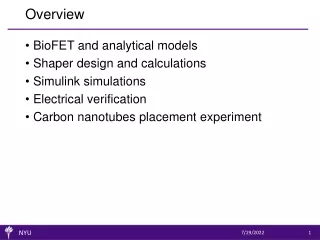
1. Overview BioFET and analytical models Shaper design and calculations Simulink simulations Electrical verification Carbon nanotubes placement experiment

2. BioFETs BioFET schematic diagram Windbacher, Thomas, et al. "Study of the Properties of Biotin-streptavidin Sensitive BioFETs." BIODEVICES. 2009. Modified by biological receptors such as HMGB1 proteins, the biosensor field-effect transistor (BioFET) can translate the number of adsorbed DNA molecules to the channel current.

3. BioFET operates in the linear region During the measurements, the BioFET operates in the linear region. Drain current is proportional to the overdrive voltage. μ is the carrier mobility, Cox is the oxide capacitance per area, W and L are the width and length of the channel, VG is the gate voltage, VT is the threshold voltage, and gm is the transconductance of the transistor.

4. Current response to analyte When analytes bind to the receptors on the surface of the BioFET gate, the surface charge density (∆q) is changed and leads to a change in the drain current. C0 is the capacitance between the channel and the analyte molecule layer. ∆q=qA[AB], where qA is the charge change caused by the unit surface density of the analyte adsorbed on the BioFET gate. [AB] representsthe surface density of adsorbed analyte molecules on the gate of BioFET.

5. Fast-mixing model In the fast-mixing model, the replenishing of the analyte from the bulk is faster than its consumption on the sensor surface. The reaction can be described as a first-order Langmuir adsorption equation. This differential equation can be solved as [A], [B] and [AB] represent the concentration of analytes in bulk solution, the surface density of functional binding sites on the sensor, and the surface density of adsorbed analyte molecules, respectively. k1 and k-1 are the association and dissociationrate constants.

6. Exponential signal Id We define and The drain current can be described as When the analyte begins to bind to the receptor, the drain current of the FET exhibits an exponential increase and the time constant τ is inversely related to the concentration [A]. We define , and the sensor responds can be described as I0 is the background current.

7.  DNA detection speed Real-time sensor responses of HMGB1–DNA binding. Duan, Xuexin, et al. "Quantification of the affinities and kinetics of protein interactions using silicon nanowire biosensors." Nature nanotechnology 7.6 (2012): 401. With a CR-RC shaper, our DNA rapid detection BioFET sensor can complete the detection of the concentration within 1s. HMGB1–DNA pair shows slow association/dissociation kinetics. It may take thousands of seconds to complete the binding and achieve equilibrium.

8. Shaper design TIA A transimpedance amplifier converts the current signal to a voltage signal. A CR-RC shaper, which contains two first-order high-pass filters and one second-order low-pass filter, converts the exponential signal to a peak shape signal. The peak value is inversely proportional to the time constant of the input signal.

9. Response calculations The transfer function of the shaper: G is the total gain of the system, PHis the pole of high-pass filter, and PL is the pole of the low-pass filter. The input signal can be expressed as

10. Response calculations We perform a Laplace transform of x(t) and calculate the response of the system.

11. Peak is proportional to 1/τ By the inverse Laplace transform, we obtain the output y(t) in time domain. Let y′(t) = 0, we have The Peak is approximately proportional to 1/τ.

12. Peak – 1/τ plot The estimated slope of Peak-1/τ plot is In our circuit, PH = 3.333, PL = 10, G=128, and I=0.25. So the estimated Slope = 2.9232. Analytical V1 = 3.1023 *1/τ + 0.0002 Estimated V2 = 2.9232 *1/τ + 0.0000 The analytical slope is calculated by Matlab.

13. Peak and [A] are linearly related Based on the previous analysis, we got Combining the two equations, we have The concentration of analyte and peak voltage are approximately linearly related.

14. Simulink simulations We verified the results we got above by using Simulink simulation. Simulink model

15. Simulink simulation results The time constant of current can be detected within 1s from the analyte and receptor start to bind. Outputs of the shaper with various τ

16. Verification steps TIA We verified the function of TIA by sending a sinusoidal signal and compare it with the output of TIA on the oscilloscope. The pole of the high-pass filter is calculated from 3dB frequency and is calibrated to 3.333. We calibrate the pole of the low-pass filter to match the outputs with the simulation results.

17. Outputs of the 1st high-pass filter Measurement results Matlab results Outputs are match with the simulation results.

18. Outputs of the 2nd high-pass filter Measurement results Matlab results Outputs are match with the simulation results.

19. Outputs of the low-pass filter Measurement results Matlab results Outputs are match with the simulation results.

20. Quantization error from NI-DAQ V Output of NI-DAQ Output of the low-pass filter The noise in the output signal is coming fromNI-DAQ. We use NIDAQ to generate the input signal with various τ:

21. External low pass filter Before external low pass filter After external low pass filter The external low-pass filter can reduce the influence of quantization noise and has almost no effect on the peak voltage.

22. Peak voltage of the shaper’s output In LPO, common mode voltage is about 0.615V. Measurement Peak = Voltage at Peak – 0.615V.

23. Peak – 1/τ plot We can calculate the τ of a given signal by measuring the peak voltage. V1 and V2 are linear fittings of measurement peak of LPO and Matlab simulation peak. The difference of intercepts is 24mV.

24. CNT selectively placement experiment CNT wrapped in SDS can self-assemble on the NMPI functionalized surface and improve the sensitivity. 4-(N-hydroxycarboxamido)-1-methylpyridinium iodide (NMPI) can self-assemble on metal oxide surfaces, but not on SiO2. Sodium dodecyl sulfate (SDS) is a surfactant of CNT,which can bind to the NMPI monolayer. Substrate with AlOx/SiO2 patterns

25. CNT solution preparation • Sonication • Centrifugation • Dialysis Break CNT aggregates. Exfoliate individual CNTs from bundles. Remove the excess SDS.

26. CNT placement Clean the substrate surface. Functionalize the substrate with NMPI. Place CNTs on the aluminum oxide surface. Annealing NMPI assembly CNT placement

27. Thanks for watching!