Introduction to Perfect Competition
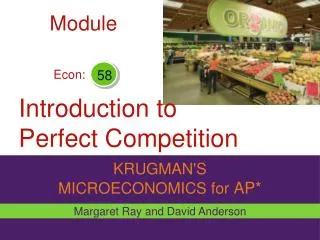
Module. Econ:. 58. Introduction to Perfect Competition. KRUGMAN'S MICROECONOMICS for AP*. Margaret Ray and David Anderson . What you will learn in this Module :. How a price-taking firm determines its profit-maximizing quantity of output.

Introduction to Perfect Competition
E N D
Presentation Transcript
Module Econ: 58 Introduction to Perfect Competition • KRUGMAN'S • MICROECONOMICS for AP* Margaret Ray and David Anderson
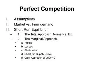
What you will learnin thisModule: • How a price-taking firm determines its profit-maximizing quantity of output. • How to assess whether or not a competitive firm is profitable. • Firms have no control over price.
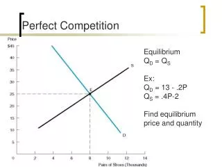
Profit Maximization in PC Optimal output rule: produce the quantity where MR=MC and profit will be maximized!
I. Production and Profits • Firms are price-takers • P = MR • MR = D = AR (Average Revenue TR/Q) • Acronym = “Mr. Darp” • Profit maximization occurs at the output level where MC = P
II. Graph Profit Maximization in PC The profit maximizing level of output is found where P = MC on the graph.
III. Calculating Profits • Total profit • π= TR – TC • If TR>TC; positive profit • If TR < TC; negative profit • Profit per unit • If P > ATC; positive profit • If P < ATC; negative profit • If P = ATC; normal profit
If it produces, a perfectly competitive firm will maximize profits at the output where: • Marginal revenue equals marginal cost • Marginal revenue equals price • Price equals average total cost • Price exceeds marginal cost • Price equals minimum average variable cost Answer: A
A competitive firm operating in the short run is producing at the output level at which ATC is at a minimum. If ATC=$8 and MR=$9, in order to maximize profits (or minimize losses), this firm should: • Increase output • Reduce output • Shut down • Do nothing; the firm is already maximizing profits • Liquidate assets and exit the industry Answer: A
Graphing Perfect Competition Module Econ: • KRUGMAN'S • MICROECONOMICS for AP* 59 Margaret Ray and David Anderson
What you will learnin thisModule: • How to evaluate a perfectly competitive firm’s situation using a graph. • How to determine a perfect competitor’s profit or loss. • How a firm decides whether to produce or shut down in the short run.
Perfect Competition Graphs How is this perfectly competitive firm doing? Is it earning a profit or a loss? MC ATC P=D
Perfect Competition Graphs • Profit maximizing output = 5 • Profit per unit is ($8 - $6) = $2 • Profit is profit per unit times the number of units. $2 x 5 = $10 MC ATC P=D
Perfect Competition Graphs A firm earning a profit. MC ATC P=D
$ MC ATC Loss ATC P P=MR=d=AR Q* Output Perfect Competition Graphs A firm experiencing a loss.
$ MC ATC P=ATC P=MR=d=AR Output Q* Perfect Competition Graphs • A firm earning a normal profit. • Also called “Break Even” price and “Break Even” point
I. The Short-run Production Decision • When a firm is earning negative profits (a loss), will it continue to produce in the short run? • Compare the losses from producing at P = MC with the losses from shutting down (producing 0) • The shut-down rule • Shut down if: • TR < TVC • P < AVC
MC $ ATC P=ATC P=MR=d=AR Output Q* Perfect Competition Graphs • The shut-down price = Point A • Any price above point A the firm will produce where P=MC AVC A Shut-down Price
II. The Long Run • When a firm is earning negative profits (a loss), in the long run, it will exit the industry. • Exit is different from shutting-down in the short run. Exit means that all fixed inputs have been sold off in the long run. The firm no longer exists. • On the other hand, if the price was consistently above the break-even price for a while, eventually new firms would want to enter the market. In the long run, new firms would be able to acquire the necessary capital inputs and join the existing firms. • Remember that under the assumptions of perfect competition, there is nothing to prevent the long-run entry or exit of firms.
The shut-down price is: • The price at which economic profit is zero • The minimum level of AVC • The intersection of the MC and ATC curves • The minimum level of AFC • Any price below ATC Answer: B
During the summer, Alex runs a lawn-mowing service, and lawn-mowing is a perfectly competitive industry. In the short run, Alex will shut down his lawn-mowing service rather than continue with it if: • The total revenues can’t cover the total fixed costs • The total revenues can’t cover the total variable costs • The total revenues can’t cover the total cost • The price exceeds the average total cost • Losses are smaller than the total fixed costs Answer: B
If price is currently between average variable cost and average total cost, then in the short run a perfectly competitive firm should: • Shut down • Continue to produce to minimize losses • Raise price • Increase production to increase profit • Reduce production to increase profit Answer: B
Long-run Outcomes in Perfect Competition Module Econ: • KRUGMAN'S • MICROECONOMICS for AP* 60 Margaret Ray and David Anderson
What you will learnin thisModule: • Why industry behavior differs between the short run and the long run. • What determines the industry supply curve in both the short run and the long run.
The Industry Supply Curve • Each identical firm’s short-run supply curve is their MC curve starting from the shut-down point (AVC curve) • The short-run supply curve for the market is the summation of the firm supply curves
I. Short Run Industry Supply Curve • The assumptions of perfect competition tell us that there are many small firms each producing an identical product. The implication of these assumptions is that each firm’s cost curves are identical as well • Individual firms supply the profit-maximizing level of output determined by their MC curve (where P = MC, above AVC) • Total output supplied in the market is equal to the output level of the firm times the number of firms in the industry.
II. Long-run Equilibrium • At the long-run equilibrium in a perfectly competitive industry, firms earn a normal profit
$ S0 S1 $8 $6 D 9000 10.000 Output $ MC $8 ATC $6 7 9 Output Long-run Adjustment Process At P = $8, P > ATC, profit, firms enter, Supply shifts right, P falls, firm Q falls.
Long Run Industry Supply Curve Cont. • When the entry of new firms does no affect the input costs in the industry it is called a constant cost industry and the long-run supply curve is horizontal • It is probably more realistic to assume an increasing cost industry. Entry of new firms increases the input costs for all firms. • it is also possible for a market to have a downward sloping LRS curve. This is when a market is a decreasing cost industry. This would occur if entry of new firms actually caused inputs to become less costly. The text provides the market for electric cars as potentially a good example. As more firms produce the cars, the infant industry of lithium batteries explodes and average costs (due to economies of scale) fall as more batteries are produced.
IV. Efficiency in Long-run Equilibrium • The perfectly competitive outcome is efficient • Productive efficiency: ATC is minimum • Allocative efficiency: P = MC • Marginal cost is the same for all producers because price is the same for all producers.
Efficiency in Long-run Equilibrium Cont. • Economic profit is equal to zero for all producers. All firms earn a normal profit in the long run. Because this can only happen at the minimum of ATC, we can say that firms produce this product at the lowest possible average cost. • The market is efficient. All consumers who are willing to pay the price that is greater than or equal to the sellers’ marginal cost will get to buy the good. In other words, there is no deadweight loss in perfect competition because all mutually beneficial transactions are made.
A curve that shows the quantity of a good or service supplied at various prices after all long-run adjustments to a price change have been completed is a long-run: • Marginal revenue curve • Marginal cost curve • Industry supply curve • Production curve • Industry demand curve Answer: C
If firms are experiencing economic losses in the short run, firms will _____ the industry and industry output will _____ and price will ______ in the long run. • exit; fall; rise • Exit; rise; fall • Enter; rise; rise • Enter; fall; rise • Exit; rise; rise Answer: A
The market for beef is in long-run equilibrium at a price of $3.25/pound. The announcement that mad cow disease has been discovered in the US reduces the demand for beef sharply, and the price falls to $2.00/pound. If the long-run supply curve is horizontal, then when long-run equilibrium is reestablished the price will be: • $3.25/pound • $2/pound • Greater than $2/pound, but less than $3.25/pound • $1.25/pound • $5.25/pound Answer: A
Introduction to Monopoly Module Econ: • KRUGMAN'S • MICROECONOMICS for AP* 61 Margaret Ray and David Anderson
What you will learnin thisModule: • How a monopolist determines the profit-maximizing price. • How to determine whether a monopoly is earning a profit or a loss. • How the monopoly outcome is different from the long-run outcome in perfect competition.
I. Monopoly Demand and MR • A Monopolist’s MR curve is below the D curve because the monopoly must lower price to sell more. • Because the monopolist is the only producer in the market, the demand for the good is the demand for the monopolist’s good
II. Profit-maximizing P and Q • A monopoly maximizes profit by producing the output level where MC = MR • The rule to maximize profit is the same, no matter the market structure
$ Profit = $12 Pm = $14 MC = ATC Pc = $10 D MR Qm= 3 Output IV. Monopoly versus Perfect Competition • Monopolies create inefficiency • P > MC • The monopolist can earn positive economic profits in the long run because there are barriers to entry of new firms
V. Monopoly vs. PC Monopoly P>MR The firm’s Demand Curve is relatively INELASTIC MR=MC The firm maximizes profit P≥ATC Long Run=Economic Profit Productive Efficiency P>Min ATC (Firm is not forced to operate with max productive efficiency) Allocative Efficiency P>MC (There is an underallocation of resources) Perfect Competition P=MR The firm’s Demand curve is Perfectly ELASTIC MR=MC The firm maximizes profit P=ATC Long Run=Normal Profit Productive Efficiency P=Min ATC (Firm is forced to operate with max productive efficiency) Allocative Efficiency P=MC (There is an optimal allocation of resources)
A monopoly is likely to _____ units of output and _____ price than a perfectly competitive firm. • Produce more; charge a higher • Produce fewer; charge a higher • Produce more; charge lower • Produce fewer; charge a lower • Produce equivalent; charge a higher Answer: B
Because monopoly firms are the only firm in the market: • They can maximize total revenue, but cannot maximize profit • They sell more at higher prices than at lower prices • They take the market-determined price as given and sell all they can at that price • They charge the highest possible price • They can only sell more by lowering price Answer: E
In the short run, a monopoly will stop producing if: • P<ATC • P<AVC • P>MR • P>ATC • P>MC Answer: B
Monopoly and Public Policy Module Econ: • KRUGMAN'S • MICROECONOMICS for AP* 62 Margaret Ray and David Anderson
What you will learnin thisModule: • The effects of monopoly on society’s welfare. • How policy-makers address the problems posed by monopoly.
I. The Welfare Effects of a Monopoly • Total surplus under perfect competition is equal to: CSc • Total surplus under monopoly is equal to: CSm + PSm • Because of the deadweight loss, we can see that CSc > CSm + PSm • What exactly is the deadweight loss? • It represents transactions (between Qc and Qm) that could have been made, but are not made under monopoly. • This will always occur when the level of output restricted such that Pm >MC. • Economists see this loss of total welfare as a major drawback to monopoly and is an argument for regulation or prevention of monopolies.