Firm behaviour
Firm behaviour . A “black box” theory of the firm – in the short run. inputs. output. cost. revenue. What do firms do?. Inputs and Cost. Production in the short run. Short-run and long-run. It can take time to adjust the level of production inputs may not be available immediately

Firm behaviour
E N D
Presentation Transcript
Firm behaviour A “black box” theory of the firm – in the short run
inputs output cost revenue What do firms do?
Inputs and Cost Production in the short run
Short-run and long-run • It can take time to adjust the level of production • inputs may not be available immediately • e.g. Parcel Delivery Company • To increase production may need to : • We will define the short and long-run by whether or not the quantity of inputs is fixed
Short run and long run • In the short run a firm can change the quantities of only some of its inputs. • In the long run a firm can change the quantities of all of its inputs. • For the moment, we’ll only study the short run.
(Short-run) production function • For now, let’s assume a firm uses only two inputs: labour and capital. • And: let’s assume labour is the variable input and capital is the fixed input. • The short-run production function shows how varying the variable input affects the quantity of output, for a given amount of the fixed input.
(Short-run) production function • Example: wheat farm • Fixed input (land): • Variable input (labour): • We’ll mostly restrict ourselves to two inputs (it’s easy). • And, we’ll usually think of land as the fixed input in the short run, • … and of labour as the variable input in the short run.
(Short-run) production function Land is fixed (10 acres)
(Short-run) production function Quantity of wheat TP Land is fixed (10 acres) Quantity of labour
Marginal product of labour Marginal product of labour Quantity of labour
Diminishing returns to an input • There are diminishing returns to an input if: • Here, there are diminishing returns to labour: • Why do we assume that the returns will begin to diminish?
Diminishing returns to an input • In our example of wheat production, the amount of land is fixed. • As the number of workers increases, the land is farmed more intensively. • This result rests on the assumption that at least one of the inputs is fixed.
From production to cost curves • Firms are only tangentially (partly) interested in the relationship between inputs and output. • To maximize profits, it would be helpful to know about the relationship between output and the cost of production. • To translate the amount of capital and labour needed to produce a given level of production to the cost of production we need to know the prices of the inputs.
(Short-run) cost • The cost that comes from the fixed input is called: • The cost that comes from the variable input is called: • The sum of fixed cost and variable cost is called total cost (TC = FC + VC).
(Short-run) cost Total cost TC Land is fixed (10 acres) Quantity of wheat
(Short-run) marginal cost • The marginal cost is the additional cost from doing one more unit of an activity. • Example (for convenience): bootmaking • Fixed cost (FC) = $108
(Short-run) marginal cost Total cost • (Short-run) total cost • (Short-run) marginal cost TC Marginal cost Quantity of boots
Explaining increasing marginal cost • Why does the short-run marginal costs increase as output expands?
(Short-run) average costs • The average fixed cost is the fixed cost per unit of output • The average variable cost is the variable cost per unit of output • The average total cost is the total cost per unit of output
(Short-run) average costs Average fixed, variable, total cost AVC AFC Quantity of boots
(Short-run) average total cost • Two effects: • “Spreading effect” • Average fixed cost falls, which tends to make average total cost fall. • “Diminishing returns effect” • Average variable cost rises, which tends to make average total cost rise.
(Short-run) ATC and MC Average total cost, marginal cost ATC Quantity of boots
(Short-run) ATC and MC • Marginal cost always goes through the minimum average total cost. • If marginal cost is below average total cost, average total cost is falling. • If marginal cost is above average total cost, average total cost is rising. • Like grades in this class!
More realistic cost curves Total cost • (Short-run) total cost • (Short-run) ATC, AVC, MC TC Marginal cost MC ATC AVC Quantity
Perfect Competition and Short-Run Supply Why unrealistic models can be useful.
Perfect competition • In a “perfectly competitive” industry: • There are many producers, each with a small market share. • Firms produce “homogeneous goods”. • There is free entry and exit • All producers are price-takers.
Production decisions • Production decisions are “how much” decisions. • We study “how much” decisions by using marginal analysis: • Compare marginal costs and marginal benefits. • Produce output up to the point where MR = MC. • This optimal output rule has got to be true for any producer.
P Market Determines Price Firm Demand: Producer’s View P q Q Price-taking and marginal revenue • Price-taking means that regardless of how much the firm produces, for each additional unit produced it gets the same price. P*
Price-taking and optimization • This implies that marginal revenue is constant. • Marginal revenue is the additional revenue from selling one more unit of output. • For price-taking producers only, the optimal output rule therefore becomes:
(Short-run) costs and MR • Example: tomato production. • Price P = $18 (MR = P).
(Short-run) MC and MR Price, marginal cost MC MR = P Quantity of tomatoes
Profit or no? • A producer makes positive profit when total revenue is greater than total cost. • TR > TC • Now divide both sides by output (Q). • TR/Q > TC/Q • So a producer is profitable when
Profit-maximizing quantity Profit (P > ATC) Price, marginal cost MC MR = P Quantity of tomatoes
Profit or loss, graphically • Profit is total revenue minus total cost: • Profit = TR – TC • Divide and multiply by output (Q): • Profit = • Profit = • Profit =
Profit-maximizing quantity Profit (P > ATC) Price, marginal cost MC MR = P ATC Quantity of tomatoes
Profit-maximizing quantity Loss (P < ATC) Price, marginal cost MC ATC MR = P Quantity of tomatoes
Profit-maximizing quantity Breaking even (P = ATC) Price, marginal cost MC ATC MR = P Quantity of tomatoes
Produce or no? • If a producer makes negative profit (a loss), will it automatically want to shut down (i.e. stop producing)? • Remember we’re in the short run! • When a producer shuts down, she still has to pay the fixed cost, so that her profit is: - FC. • That is, a producer wants to shut down only if:
Produce or no? • Shut down if: • Profit (producing) < profit (shutting down) • TR – (VC + FC) < 0 – FC • < • < • < • <
Produce, with profit Price, marginal cost MC MR = P ATC AVC Quantity of tomatoes
Produce, with loss Price, marginal cost MC ATC AVC MR = P Quantity of tomatoes
Profit-maximizing quantity Shut-down price Price, marginal cost MC ATC AVC MR = P Quantity of tomatoes
Shut-downprice Summary of producer decisions Price, marginal cost MC ATC AVC Quantity of tomatoes
Summary of producer decisions • The short-run individual supply curve summarizes the production (“supply”) decisions of one individual, perfectly competitive, producer. • The short-run industry supply curve summarizes the supply decisions by all producers in a perfectly competitive industry.
Individual and industry S curves Price • Short-run individual supply curve • Short-run industry supply curve … • … when the industry consists of 100 producers • “Market supply curve” Price S Quantity of boots

