Download
1 / 29
290 likes | 469 Vues
Earth Observation Data and Carbon Cycle Modelling. Marko Scholze QUEST, Department of Earth Sciences University of Bristol GAIM/AIMES Task Force Meeting, Yokohama, 24-29 Oct. 2004. (an incomplete and subjective view…). Overview. Atmospheric CO 2 observations TransCom

E N D
Earth Observation Data and Carbon Cycle Modelling Marko Scholze QUEST, Department of Earth Sciences University of Bristol GAIM/AIMES Task Force Meeting, Yokohama, 24-29 Oct. 2004 (an incomplete and subjective view…)
Overview • Atmospheric CO2 observations • TransCom • Model-Data Synthesis • Oceanic DIC observations: Inverse Ocean Modelling Project • Terrestrial observations: Eddy-flux towers • Atmospheric observations: Carbon Cycle Data Assimilation system
TransCom 3 Linear atmospheric transport inversion to calculate CO2 sources and sinks: • 4 background "basis functions" for land, ocean, fossil fuels 1990 & 1995 • 11 land regions, spatial pattern proportional to terr. NPP • 11 ocean regions, uniform spatial distribution • Solving for 4 (background) + 22 (regions) * 12 (month) basis functions!
TransCom 3 Seasonal Results(mean over 1992 to 1996) Guerney et al., 2004 inversion results: response to background fluxes: 15 4 Gt C/yr -5 -35 ppm
TransCom 3 Interannual Results (1988 - 2003) red: land blue: ocean darker bands: within-model uncertainty lighter bands: between- model uncertainty Gt C/yr • larger land than ocean variability • interannual changes more robust than seasonal ... but atmosphere well mixed interannually... Baker et al. 2004
Model-Data Synthesis:The Inverse Ocean Modelling Project Recent ocean carbon survey, ~ 60.000 observations C* of Gruber, Sarmiento, and Stocker (1996) to estimate anthropogenic DIC. Innumerable data authors, but represented by Feely, Sabine, Lee, Key.
The Inverse Ocean Modelling Project Jacobson, TransCom3 Meeting, Jena, 2003
The Inverse Ocean Modelling Project • southward carbon transport of 0.37 Pg C/yr for pre-industrial times • present-day transport -0.06 Pg C/yr (northwards) Gloor et al. 2003
Terrestrial observations: Fluxneta global network of eddy covariance measurements Inversion of terrestrial ecosystem parameter values against eddy covariance measurements by Metropolis Monte Carlo sampling
A Posteriori parameter PDF for Loobos site ga,v: vegetation factor of atmospheric conductance Evm: activation energy of Vm Knorr & Kattge, 2004
Carbon sequestration at the Loobos site during 1997 and 1998 Knorr & Kattge, 2004
CCDASCarbon Cycle Data Assimilation System Misfit 1 CO2 station concentration InverseModeling: Parameter optimization Fluxes Model parameter ForwardModeling: Parameters –> Misfit Misfit to observations Atmospheric Transport Model: TM2 Biosphere Model: BETHY
CCDAS set-up 2-stage-assimilation: • AVHRR data (Knorr, 2000) • Atm. CO2 data Background fluxes: • Fossil emissions (Marland et al., 2001 und Andres et al., 1996) • Ocean CO2(Takahashi et al., 1999 und Le Quéré et al., 2000) • Land-use (Houghton et al., 1990) Transport Model TM2(Heimann, 1995)
Methodology where • is a model mapping parameters to observable quantities • is a set of observations • error covariance matrix Uncertainties of prognostics X Uncertainties of parameters need of (adjoint of the model) Minimize cost function such as (Bayesian form):
Gradient Method cost function J (p) 1st derivative (gradient) of J (p) to model parameters p: yields direction of steepest descent. 2nd derivative (Hessian) of J (p): yields curvature of J. Approximates covariance of parameters. Model parameter space (p) Figure from Tarantola, 1987
Seasonal Cycle Barrow Niwot Ridge observed seasonal cycle optimised modeled seasonal cycle
Global Growth Rate observed growth rate optimised modeled growth rate Atmospheric CO2 growth rate Calculated as:
Error Reduction in Parameters Relative Error Reduction
Carbon Balance Euroflux (1-26) and other eddy covariance sites* latitude N *from Valentini et al. (2000) and others net carbon flux 1980-2000 gC / (m2 year)
IAV and processes Major El Niño events Major La Niña event Post Pinatubo period
Interannual Variability Normalized CO2 flux and ENSO Lag correlation (low-pass filtered) correlation coefficient
Outlook • Data assimilation: problem better constrained without "artefacts" (e.g. spatial patterns created by station network) but: cannot resolve processes that are not included in the model (look at residuals and learn about the model) • Simultaneous inversion of land and ocean fluxes • Isotopes • More data over tropical lands: satellites • Model-Data-Synthesis: problem better constrained without "artefacts" (e.g. spatial patterns created by station network) but: cannot resolve processes that are not included in the model (look at residuals and learn about the model) • Simultaneous inversion of land and ocean fluxes • Further data constraints (e.g. Isotopes, Inventories) • More data over tropical lands: satellites
Posterior Uncertainty in Net Flux Uncertainty in net carbon flux 1980-200 gC / (m2 year)
Uncertainty in prior net flux Uncertainty in net carbon flux from prior values 1980-2000 gC / (m2 year)
Atm. Inversion on Grid-cell Rödenbeck et al. 2003 • prior and posterior uncertainties • sensitivities (colors)
Atm. Inversion on Grid-cell Not really at model grid of TM3, but aggregated to TM2 grid, 8° x 10°, Underdetermined problem correlation matrix (e.g. l=1275 km for NEE) prior/posterior fluxes and reduction in uncertainty Rödenbeck et al. 2003
CO2 Satellite Measurements Sciamachy, OCO Airs (U) (=Upper limit) Airs (L) (=Lower limit) Vertical weighting functions Houweling et al. 2003
Pseudo Satellite Data Inversion posterior/prior uncertainty Houweling et al. 2003