Jim Demmel EECS & Math Departments, UC Berkeley demmel@cs.berkeley.edu

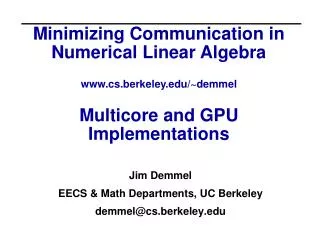
Minimizing Communication in Numerical Linear Algebrawww.cs.berkeley.edu/~demmelMulticore and GPU Implementations Jim Demmel EECS & Math Departments, UC Berkeley demmel@cs.berkeley.edu

Outline of Dense Linear Algebra • Multicore implementations • DAG Scheduling to minimize synchronization • Optimization on GPUs • Minimizing data movement between CPU and GPU memories Summer School Lecture 5

Multicore: Expressing Parallelism with a DAG for k = 0 to N-1 for n = 0 to k-1 A(k,k) = A(k,k) – A(k,n)*A(k,n) A(k,k) = sqrt(A(k,k)) for m = k+1 to N-1 for n = 0 to k-1 A(m,k) = A(m,k) – A(m,n)*A(k,n) A(m,k) = A(m,k) / A(k,k) • DAG = Directed Acyclic Graph • S1  S2 means statement S2 “depends on” statement S1 • Can execute in parallel any Si without input dependencies • For simplicity, consider Cholesky A = LLT, not LU • N by N matrix, numbered from A(0,0) to A(N-1,N-1) • “Left looking” code CS267 Lecture 11

Expressing Parallelism with a DAG - Cholesky for k = 0 to N-1 for n = 0 to k-1 A(k,k) = A(k,k) – A(k,n)*A(k,n) A(k,k) = sqrt(A(k,k)) for m = k+1 to N-1 for n = 0 to k-1 A(m,k) = A(m,k) – A(m,n)*A(k,n) A(m,k) = A(m,k) · A(k,k)-1 S1(k,n) S2(k) S3(k,m,n) S4(k,m) n S1(k,n) DAG has N3/6 vertices: S1(k,n)  S2(k)for n=0:k-1 S3(k,m,n) S4(k,m)for n=0:k-1 S2(k) S4(k,m)for m=k+1:N S4(k,m) S3 (k’,m,k)for k’>k S4(k,m) S3(k,m’,k) for m’>m k S2(k) S3(k,m,n) S4(k,m) m CS267 Lecture 11

Expressing Parallelism with a DAG – Block Cholesky • Each A[i,j] is a b-by-b block SYRK: POTRF: GEMM: TRSM: for k = 0 to N/b-1 for n = 0 to k-1 A[k,k] = A[k,k] – A[k,n]*A[k,n]T A(k,k) = unblocked_Cholesky(A(k,k)) for m = k+1 to N/b-1 for n = 0 to k-1 A[m,k] = A[m,k] – A[m,n]*A[k,n]T A(m,k) = A(m,k) · A(k,k)-1 S1(k,n) S2(k) S3(k,m,n) S4(k,m) n S1(k,n) k S2(k) Same DAG, but only (N/B)3/6 vertices S3(k,m,n) S4(k,m) m CS267 Lecture 11

Sample Cholesky DAG with #blocks in any row or column = N/b = 5 Slide courtesy of Jakub Kurzak, UTK Note implied order of summation from left to right Not necessary for correctness, but it does reflect what the sequential code does Can process DAG in any order respecting dependences CS267 Lecture 11

Scheduling options • Static (pre-assign tasks to processors) or Dynamic (idle processors grab ready jobs from work-queue) • If dynamic, does scheduler take user hints/priorities? • Respect locality (eg processor must have some task data in its cache) vs not • Build and store entire DAG to schedule it (which may be very large, (N/b)3 ), or build just the next few “levels” at a time (smaller, but less information for scheduler) • Programmer builds DAG & schedule vs depending on compiler or run-time system • Ease of programming, vs not exploiting user knowledge • If compiler, how conservative is detection of parallelism? Summer School Lecture 5

Schedulers tested • Cilk • programmer-defined parallelism • spawn – creates independent tasks • sync – synchronizes a sub-branch of the tree • SMPSs • dependency-defined parallelism • pragma-based annotation of tasks (directionality of the parameters) • PLASMA (Static Pipeline) • programmer-defined (hard-coded) • apriori processing order • progress tracking • stalling on dependencies Slide courtesy of Jakub Kurzak, UTK

Measured Results for Tiled Cholesky PLASMA: • Measured on Intel Tigerton 2.4 GHz • Cilk 1D: one task is whole panel, but with “look ahead” • Cilk 2D: tasks are blocks, scheduler steals work, little locality • PLASMA works best Summer School Lecture 5 Slide courtesy of Jakub Kurzak, UTK

More Measured Results for Tiled Cholesky • Measured on Intel Tigerton 2.4 GHz Cilk SMPSs PLASMA (Static Pipeline) Slide courtesy of Jakub Kurzak, UTK

Still More Measured Results for Tiled Cholesky • PLASMA (static pipeline) – best • SMPSs – somewhat worse • Cilk 2D – inferior • Cilk 1D – still worse quad-socket, quad-core (16 cores total) Intel Tigerton 2.4 GHz Slide courtesy of Jakub Kurzak, UTK

Intel’s Clovertown Quad Core 3 Implementations of LU factorization Quad core w/2 sockets per board, w/ 8 Threads 3. DAG Based (Dynamic Scheduling) 2. ScaLAPACK (Mess Pass using mem copy) 1. LAPACK (BLAS Fork-Join Parallelism) 8 Core Experiments Source: Jack Dongarra

Scheduling on Multicore – Next Steps • PLASMA 2.0.0 released • Just Cholesky, QR, LU, using static scheduling • LU does not do partial pivoting – Stability? • http://icl.cs.utk.edu/plasma/ • Future of PLASMA • Add dynamic scheduling, similar to SMPSs • DAGs for eigenproblems are too complicated to do by hand • Depend on user annotations and API, not compiler • Still assume homogeneity of available cores • What about GPUs, or mixtures of CPUs and GPUs? • MAGMA Summer School Lecture 5

QR Factorization Intel 16 coresTall Skinny Matrices Gflop/s N, where matrix is M=51200 x N Summer School Lecture 5

LAPACK QR . . . Step 1 Step 2 Step 3 Step 4 Summer School Lecture 5

Parallel Tasks in QR Break into smaller tasks and remove dependencies Summer School Lecture 5

Parallel Tasks in QR Step 1: QR of block 1,1 Summer School Lecture 5

Parallel Tasks in QR Step 1: QR of block 1,1 Step 2: Use R to zero A1,2 Summer School Lecture 5

Parallel Tasks in QR Step 1: QR of block 1,1 Step 2: Use R to zero A1,2 Step3: Use R to zero A1,3 . . . Summer School Lecture 5

QR Factorization Intel 16 coresTall Skinny Matrices Gflop/s N, where matrix is M=51200 x N Summer School Lecture 5

Communication Reducing QR Factorization • TS matrix • MT=6 and NT=3 • split into 2 domains • 3 overlapped steps • panel factorization • updating the trailing submatrix • merge the domains Summer School Lecture 5

Communication Reducing QR Factorization • TS matrix • MT=6 and NT=3 • split into 2 domains • 3 overlapped steps • panel factorization • updating the trailing submatrix • merge the domains • Final R computed Summer School Lecture 5

Example with 4 and 8 Domains A. Pothen and P. Raghavan. Distributed orthogonal factorization. In The 3rd Conference on Hypercube Concurrent Computers and Applications, volume II, Applications, pages 1610–1620, Pasadena, CA, Jan. 1988. ACM. Penn. State. Summer School Lecture 5

Execution Trace 16 core run Summer School Lecture 5

Communication Reducing QR Factorization Quad-socket, quad-core machine Intel Xeon EMT64 E7340 at 2.39 GHz. Theoretical peak is 153.2 Gflop/s with 16 cores. Matrix size 51200 by 3200 Sequential PLASMA

Cluster Experiment • grig.sinrg.cs.utk.edu • 61 nodes • Two CPUs per node • Intel Xeon 3.20GHz • Peak performance 6.4 GFLOPS • Myrinet interconnection (MX 1.0.0) • Goto BLAS 1.26 • DGEMM performance 5.57 GFLOPS (87%) • MPICH-MX • gcc 64 bits Summer School Lecture 5 Courtesy Jack Dongarra

Weak Scalability (8 columns of tiles) Courtesy Jack Dongarra

Weak Scalability (8 columns of tiles) On 1 CPU, the matrix size is 64x8 tiles On k CPUs, the matrix size is k*64x8 tiles Tiles are 200x200 blocks Courtesy Jack Dongarra

Weak Scalability (8 columns of tiles) Courtesy Jack Dongarra

Dense Linear Algebra on GPUs • Source: Vasily Volkov’s SC08 paper • Best Student Paper Award • New challenges • More complicated memory hierarchy • Not like “L1 inside L2 inside …”, • Need to choose which memory to use carefully • Need to move data manually • GPU does some operations much faster than CPU, but not all • CPU and GPU like different data layouts Summer School Lecture 5

Motivation • NVIDIA released CUBLAS 1.0 in 2007, which is BLAS for GPUs • This enables a straightforward port of LAPACK to GPU • Consider single precision only • Goal: understand bottlenecks in the dense linear algebra kernels • Requires detailed understanding of the GPU architecture • Result 1: New coding recommendations for high performance on GPUs • Result 2: New , fast variants of LU, QR, Cholesky, other routines

GPU Memory Hierarchy • Register file is the fastest and the largest on-chip memory • Constrained to vector operations only • Shared memory permits indexed and shared access • However, 2-4x smaller and 4x lower bandwidth than registers • Only 1 operand in shared memory is allowed versus 4 register operands • Some instructions run slower if using shared memory

Memory Latency on GeForce 8800 GTXRepeat k = A[k] where A[k] = (k + stride) mod array_size

Jim Demmel EECS & Math Departments, UC Berkeley demmel@cs.berkeley.edu