Download
1 / 20
200 likes | 522 Vues
SGR 1806-20 Giant Flare and Gravitational Wave emission. Coincidences data analysis using cross correlation techniques. SGR 1806-20 Giant Flare. 27 Dec. 2004 Giant Flare SGR 1806-20 Double structure: precursor (at -142 s.) and flare

E N D
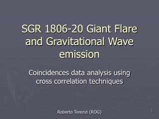
SGR 1806-20 Giant Flare and Gravitational Wave emission Coincidences data analysis using cross correlation techniques Roberto Terenzi (ROG)
SGR 1806-20 Giant Flare • 27 Dec. 2004 Giant Flare SGR 1806-20 • Double structure: precursor (at -142 s.) and flare • Search for gravitational wave emission (gwe) in coincidences with flare and precursor Roberto Terenzi (ROG)
Flare and precursor (from Nature) - ±10s, i.e. ±10s, i.e. ±10s, i.e.
Data Analysis: coincidences between electromagnetic emission and gwe • Coincidences windows=± 10 s (Magnetar spin period=7.56s, see Nature) • Both at flare and at precursor • Analysis technique : cross correlation coefficient • For two sets of data {x} and {y}: Roberto Terenzi (ROG)
Cross correlation coefficient parameters settings • Lag: it depends on time of fly and detectors electronics delays. • Correlation interval: it depends on signal time length (1s.) • Correlation step (k): it depends on how much time resolution in cross correlation coefficients we would like to have (20 ms) Roberto Terenzi (ROG)
Time of fly and lag • A gravitational wave (gw) coming from the Magnetar on the 27 Dec. 2004 at 21h:30m:26.68s should hit first Explorer and then Nautilus with a time delay of the order of 1250 μs. • In Dec. 2004 the Explorer and Nautilus electronics are different: they present an input-output signal difference in delay time of the order of 650 μs . • Nominal lag= (1250-650) ± 300 μs., direction: Explorer data sequence should be delayed before cross correlate with Nautilus data sequence of about 600μs ± 300 μs due to data timing uncertainties Roberto Terenzi (ROG)
Data • 1. Detector output data orraw data: data collected at the end of the detector electronics acquisition chain, without any further conditioning. • 2. Detector input data orinput data or deconvolved data: the detector output data deconvolved by the detector transfer function to get the input strain h. • 3. White or whitened data: the output of a whitening process on the input data that re-normalize the noise. • 4. Filtered or wavelets filtered data: the output of an EWF applied to the whitened data. Roberto Terenzi (ROG)
Input Data Roberto Terenzi (ROG)
Data Analysis Pipeline 1 data flow • 1. Detectors raw data deconvolved by detectors transfer function input data (h) • 2. Input data spectrum module averaged reference whitening spectrum • 3. Chunk of input data divided by reference whitening spectrum whitened data • 4. Whitened data filtered by EWF filtered data • 5. Filtered data Cross correlation coefficients (ccc) Roberto Terenzi (ROG)
Data Analysis Pipeline 2.1:ccc data processing • Q.: In a ± 10s coincidence window how the candidate coincidence timing between electomagnetic emission and gwe can be defined? • A.: With 1 detector only, by choosing the time of the maximum of the signal in the window, for example. With two detectors….. Roberto Terenzi (ROG)
Data Analysis Pipeline 2.2 • A.: With TWO detectors, we can select the time of the 1s sub-interval showing the maximum cross correlation coefficient between the two detectors data. Roberto Terenzi (ROG)
Data Analysis Results 4: Cross Correlation coefficient values:4h data, 200ms Roberto Terenzi (ROG)
Data Analysis Results 1: Cross Correlation coefficient values Roberto Terenzi (ROG)
Data Analysis Results 3: Cross Correlation coefficient values Whitened and Filtered data Roberto Terenzi (ROG)
Data Result: 0.275,0.282 ?? • Statistics on ccc: • 4 hours of data cross correlated • Histogram and Gaussian Fit • Frequency of occurrence of data value found in the distribution fit • Probability, given the two values, of having such values in the 2 coincidences windows • ENERGY of gwe needed to have such values (i.e. method calibration) Roberto Terenzi (ROG)
Data Analysis Results 5: Max of Cross Correlation coefficient values in 4h data ± 10 s coincidence windows Roberto Terenzi (ROG)
Data Analysis Results 5: Max of Cross Correlation coefficient values in 4h data ± 10 s coincidence windows Roberto Terenzi (ROG)
Data Result: 0.275,0.282 ?? • Statistics on ccc: • 4 hours of data cross correlated • Histogram and Gaussian Fit • Frequency of occurrence of data value found in the distribution fit • Probability, given the two values, of having such values in the 2 coincidences windows • ENERGY of gwe needed to have such values (i.e. method calibration) Roberto Terenzi (ROG)
Data Result: 0.275,0.282 ?? • Frequency of occurrence of data value found in the distribution fit: 3.38σ and 3.58σ • Probability, given the two values, of having such values in the 2 coincidences windows: p≈10^−5 Roberto Terenzi (ROG)
Data Result: 0.275,0.282 ?? • ENERGY of gwe needed to have such values (at precursor, hip: Magnetar at 15kpc): 7 ∗ 10^−4 M c^2 M= Solar mass Less at flare… Roberto Terenzi (ROG)