Download
1 / 27
300 likes | 690 Vues
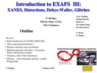
Introduction to EXAFS III: XANES, Distortions, Debye-Waller, Glitches. Scott Medling Michael Kozina Brad Car Yu (Justin) Jiang Lisa Downward C. Booth G. Bunker. F. Bridges Physics Dept. UCSC, MC2 Chalmers. Outline Review Brief introduction to XANES (NEXAFS)

E N D
Introduction to EXAFS III: XANES, Distortions, Debye-Waller, Glitches Scott Medling Michael Kozina Brad Car Yu (Justin) Jiang Lisa Downward C. Booth G. Bunker F. Bridges Physics Dept. UCSC, MC2 Chalmers Outline • Review • Brief introduction to XANES (NEXAFS) • Why understand distortions ? • Phonon vibrations and correlations • Modeling thermal vibrations : Correlated Debye and Einstein models • Polarons, Jahn-Teller distortions • Glitches – monochromator glitches, sample Bragg peaks. Chalmers 2011
Review - EXAFS Equations Fi(k,r), c , i --calculated using FEFF σi – width of pair distribution function, g(ro,i,r) Ai= Ni So2 (ħk)2/2m = E-Eo Simplify to first neighbor peak only (we will fit in r-space – Fourier transform space) Use either: FEFF to generate a theoretical standard (calculate Fi(k,r), c , i ) or an experimental standard Experimental standard Chalmers 2011
XANES Region around edge; typical up to 30 eV above, but can be higher. Includes small pre-edge features at bottom of edge. “White” line at top of edge varies with environment – from film days, high intensity line would make film “white” on photo. Chalmers 2011
How do you describe XANES? Same matrix elements – dominated by electric dipole transitions, Δℓ = ± 1, but small quadrupole transition sometimes in in pre-edge. K-edges , 1s → np ; often mixture (hybridization) of states on neighboring atoms. L3, L2 edges, 2p → nd or ms; 2p → nd dominate. Dipole Quadrupole Chalmers 2011
Final state of photoelectron difficult to determine Problem: is it localized (atomic-like), or extended (band-like) ; should it be treated as a scattering process rather than localized or band states ? Complex theoretical problem Edge position – usually depends on valence and local environment – bond lengths and symmetry. Only Qualitative agreement between theory and experiment (numerical calculation are intensive). No theoretical model to do direct fit of XANES -- EXAFS can do quantitative fits J. SOLID STATE CHEM 141 294-297 (1998) Structure in edge – depends on environment – often little structure for small clusters/molecules. More XANES structure as make cluster large (FEFF8 -- scattering approach) and include multiple scatterings. LiMn2O4 FEFF calculations for Mn K-edge Chalmers 2011
Other considerations • Core-hole life time 10-15 sec. Some other electron drops into core-hole and emits a fluorescence photon – ends the process. Entire absorption and multi-scattering of photo-electron takes place within life time. Locally the lattice is frozen on this time scale. • Core-hole lifetime becomes shorter for higher Z - by uncertainty principle short life time gives an energy broadening of spectra. At Cu edge (9 keV) a few eV, but at high Z, (I or Ba) large broadening. Resonant Inelastic X-ray Scattering (RIXS) can partially avoid this broadening. • White lines, particularly for L edges, can be very high and can distort fluorescence data (self-absorption); also important to have small particles because if particle size is too large, it distorts white line. Particle diameter < absorption length. Chalmers 2011
Empirical approaches • Edges shift with increasing valence (same number of neighbors) for K edges 3-4 eV per valence unit for L3 edges can be larger 7eV/unit • Shift appears to be mainly a bond length change – higher valence, shorter the bond length. Estimates of charge transfer are quite small. • Edge positions differ for different configurations -- tetrahedral vs octahedral. • For mixed samples (geological) - may be a sum of known compounds. If have good XANES for the references, can fit data to a weighted sum of reference files. Often works well, - can provide relative abundances quickly. Requires that you know all compounds -- if missing one results aren’t reliable. • Principal component analysis • Based on linear algebra; treat each XANES spectra as a vector. Can one find a set of vectors (components) such that data is a linear weighted sum of the component? Turns out YES – and can find a minimum number - robust. Chalmers 2011
Distortions -- Motivation • All systems have local distortions from lattice vibrations. In large-unit-cell systems an atom may be weakly bonded to the rest of the crystal – can have large vibration amplitudes – called a “rattler”. This disorder can strongly scatter thermal phonons and lead to a glass-like, low thermal conductivity. • Some systems have a Jahn-Teller (JT) distortion– e.g. the six O atoms around Mn+3 in LaMnO3 are not equivalent; there is a distortion with two long bonds and 4 shorterbonds (the four are slightly split). A similar JT splitting is expected for Cu2+. In contrast for CaMnO3, the 6 Mn+4-O bonds are equal within 0.01Ǻ. The competition between distorted and undistorted sites determines the magnetic and transport properties in substituted manganites (La1-xCaxMnO3) which are metallic and ferromagnetic at low T for some concentrations x, but non-metallic and insulating at high T. • All these properties require knowledge about the broadening of the atom-pair distribution functions – usually described in terms of the width σ. σ2 = sum over all broadening mechanisms Chalmers 2011
Thermal vibrationsSimple example – isolated atom pair Use reduced mass – MR = 1/2m x is the variation in the bond length, about r0 κ is the spring constant only one mode of vibration -- Einstein model m m at high T κ = MRω2 ħω = kBΘ zero-point motion Chalmers 2011
Split peaks and σ When one has an unresolved split peak (i.e. small splittings) it contributes to the broadening (See EXAFS book by B. Teo); easiest to see at low T. r ~π/(2kmax) to resolve Equal splitting of 6 bonds into two groups (3+3) split by Δr; and each split peak has same σj δ(σ2) = (Δr/2)2 ; σone peak fit = σj2 + (Δr/2)2 Splitting into three peaks with equal splittings, Δr. Then δ(σ2)= ((2/3)Δr)2 Chalmers 2011
Different Phonon Modes http://physics.ucsc.edu/~bridges/simulations/index.html Long Wavelength Acoustic Phonon Positive correlations Short Wavelength Optical Phonon Negative correlations Motions of neighboring atoms are correlated in dynamical examples Polaron transportation Chalmers 2011
Debye-Waller factors, Diffraction, and Correlations • Important: EXAFS measures MSD differences in position (in contrast to diffraction!!) • Harmonic approximation: Gaussian Pi Pj • Ui2 are the position mean-squared displacements (MSDs) from diffraction • Φ is the correlation factor – can be positive or negative.
Comparison between Einstein and Correlated Debye models – T Dependence I(Simple systems) Correlated Debye Model (All modes; sometimes restricted to Acoustic modes) Einstein model (local modes, optical modes) Rijis for atom pair ij MR – reduced mass κ– Spring constant ΘE– Einstein Temperature ΘcD– Correlated Debye Temperature; ΘcD =ℏωcD/kB c – effective speed of sound = ωcD/kD • At T~0, σ2E(0) = ħ2/(2MRkBΘE) • = kBΘE/(2κ) Chalmers 2011
Einstein, ΘE = 750K Debye model, ΘD = 950K Einstein, ΘE = 950K Temperature Dependence of σ2 Einstein vs Correlated Debye • Some general properties: • For thermal vibrations σ2thermalvs T has a positive slope; linear with T at high T. Einstein model has a sharper bend with T. • Zero-point motion determines σ2thermalat low T – for Einstein Model, should correlate with appropriate Raman mode . • If static disorder present (σ2static), produces a rigid vertical shift [σ2 = σ2static + σ2thermal]. Chalmers 2011
Other types of distortions • Contributions to 2 • Thermal phonons – Einstein or Debye models. • Static distortions – distribution of pair distances from strains, impurities, etc. • Polarons – a distortion associated with a partially localized charge. • Jahn-Teller distortions e.g. Mn+3, Cu+2 • Off-centerdisplacements (ferroelectric) • Dynamic distortions – time scale? Polaron Distortion produced by charged carrier and follows carrier; dynamic. Can move very fast if charge carrier moves rapidly. If too fast, lattice response is small. For uncorrelated mechanisms: σ2total= σ2thermal+ σ2static +σ2polarons+ σ2JT+ σ2off Chalmers 2011
The Jahn-Teller (JT) Distortion • JT distortions lead to a distribution of Mn-O (or Co-O) bond lengths. • Mn3+ (LaMnO3) has 3d4 configuration – one eg elect. • The oxygen displacements about Mn3+for a Jahn–Teller distortion are indicated by arrows • Assumes one quasi-localized eg electron is present on Mn; localized for times long compared to optical phonon period (~10-13 sec.). • Mn4+, 3d3 config., (CaMnO3) - no eg electrons, no JT. • (What happens for La1-xCaxMnO3??) • Cu+ - 3d10 ; Cu+2 - 3d9, JT active • Simplified energy level diagram; eg and t2g split by crystal field. • Large exchange energy (Hubbard U), so each level can only be singly occupied. • For only one egelectron, a JT distortion of the surrounding O6 octahedron can occur spontaneously; this splits the egdoublet by an energy EJT, and lowers total energy by ΔE = -EJT/2 +Estrain • If ΔE < 0, Jahn-Teller distortions form. A.J. Millis, Nature 392, 147 (1998) UCSC April 2011
Spikes/peaks in EXAFS data that are not part of EXAFS oscillations • Some obvious, others not; change shape of EXAFS k-space/r-space data and can introduce significant error. • Several causes • Harmonics in X-ray beam or non-uniform samples + • multiple diffraction in monochromator crystals . • Bragg diffraction from sample (single crystal , crystal substrate, or oriented thin film). • Need to be able to minimize and/or remove them Glitches in EXAFS spectra Only important when diffraction is possible, and peaks relatively large. Usually not important for soft X-rays < 2 keV; (depends on crystal). Glitches also become very small at high energies E > 20-25 keV. Chalmers 2011
Monochromator Glitch library (SSRL) http://www-ssrl.slac.stanford.edu/userresources/index.html Changes in Io intensity as scan energy Quite extensive library for 111 and 220 crystals Covers range from 2.5 to ~ 23 keV for some crystals In practice we choose mono-crystals that have the lowest amplitude glitches in the energy range for our samples. Si(220) phi=0 (SSRL BL 7-3) Si(220) phi=90 (SSRL BL 7-3) Chalmers 2011
Examples of multiple diffractionsin 2-D (exist in 3-D) Ewald sphere in K-space 2d sin θ = nλ; k = 2π/λ Incident beam Desired monochromator Bragg planes Other sets of planes (Blue and Green) that meet Bragg condition over a tiny rotation angle Chalmers 2011
Glitches -Variations in ln(Io/I1):Harmonics or non-uniform sample Bragg scattering: 2dsinθ = nλ n= 1 fundamental; n > 1 harmonics Assume no harmonics, and uniform t I1 = Ioe-µt µt = ln(Io/I1) Non-uniform t - consider i elements: µti = ln(Ioi/I1i) for each element Harmonics present – IH Usually 2nd (220’s) or 3rd (111) are main harmonics. Intensity above 30 keV small Io = Io' + IH ; IH/ Io ' small. I1 = Io'e-µt + α IH ln(Io/I1) ≈ µt + IH/ Io'(1- αeµt) Chalmers 2011
Examples of glitches in unfocused beam:multiple diffractions Typical slits; slope of intensity varies as glitch passes. These data collected with small slits 0.2mm Expanded view of large glitch – subtracted scan at 6765 eV from rest of scans Chalmers 2011
Coupling between Beam Intensity non-uniformity and sample non-uniformity The signal obtained from a detector is an integral over the cross-sectional area of the beam. F(x,y,E) is the X-ray flux (I/area) slit width a, slit height b μ(E) absorption coefficient t(x,y) sample thickness. Simple case: One dimension and assume F(y,E) and t(y) vary linearly with y; t(y ) = to(1 + αy); F(y,E) = Fo(E)(1 + βy) and μ(E)to αy <<1; exp(-μ(E)toαy) ~ (1- μ(E)toαy) Non-uniformities couple when both Io and t vary spatially For small α and β, correction 10-3 to 10-4 Chalmers 2011
Wedge plexiglas sample; t(y) = 1.5 +0.2y ( 1 mm slit, t(y) varies from 1.4 to 1.6 mm) Dotted lines in (b) show model Pinholes and tapers Single pinhole in foil. Nucl. Instr. & Meth. A320, 548 (1992). Wedge up Wedge down Note sign change. Sum of +y and –y is almost zero. Uniform distribution of tiny pinholes has low glitch amplitude. GG. Li etal. Nucl. Instr. & Meth. A340, 420 (1994) Chalmers 2011
Minimizing Glitches • Make samples as uniform as possible; small variation in thickness and few pinholes. • Eliminate harmonics (harmonic rejection mirror or “detuning” mono) • Use narrow vertical slits -- reduces glitch amplitude and can improve energy resolution. • Use different monochromator crystals • If you have significant glitches, you have a non-uniform sample or significant harmonic contamination • Small, narrow glitches (1-3 points) can be removed; but be careful Chalmers 2011
Sample glitches: single crystals, thin films • For anisotropic single crystals or thin films may want to do polarized EXAFS with E polarization along different crystal axes or directions; usually detect using fluorescence. • Over a typical EXAFS scan, usually several Bragg diffractions from sample – reduced absorption in sample. These move if sample is rotated slightly. Series of data sets at several slightly different angles, usually allows removal but time consuming. • For thin films, if incident beam is Bragg scattered from substrate and passes through sample again – get increased fluorescence. Again will move if sample is rotated slightly. Don’t use single crystals of cubic materials, use powders! Chalmers 2011
More caveats II • Don’t go too low in k-space in choosing the FT range. Remember k = 0.512 (E-Eo)½; so for k = 3 Å-1 , E-Eo= 34.3 eV, and for k = 2 Å-1, E-Eo= 15.3 eV. XANES structure usually extends up to 20-30 eV above edge and sometimes higher, so dangerous to go below k = 3 Å-1. If not sure, do fits for various FT ranges -- parameters should not change significantly. If large change in σ, say from kmin = 2.5 and 3 Å-1 then a problem. • Strong correlations between N and σ. Don’t think of σ as a “throw-away” parameter, even when you are more interested in N and r. σ must be larger than zero-point motion value. • kn weighting; depends on backscattering atom. Usually k2 or k3 make EXAFS spectra sharper – but be careful of noise at high k. Chalmers 2011
Further reading • Thickness effect: Stern and Kim, Phys. Rev. B 23, 3781 (1981). • Particle size effect: Lu and Stern, Nucl. Inst. Meth. 212, 475 (1983). • Glitches: • Bridges, Wang, Boyce, Nucl. Instr. Meth.A 307, 316 (1991); Bridges, Li, Wang, Nucl. Instr. Meth. A 320, 548 (1992);Li, Bridges, Wang, Nucl. Instr. Meth. A 340, 420 (1994). • Number of independent data points: Stern, Phys. Rev. B 48, 9825 (1993); Booth and Hu, J. Phys.: Conf. Ser. 190, 012028(2009). • Theory vs. experiment: • Li, Bridges and Booth, Phys. Rev. B 52, 6332 (1995). • Kvitky, Bridges, van Dorssen, Phys. Rev. B 64, 214108 (2001). • Polarized EXAFS: • Heald and Stern, Phys. Rev. B 16, 5549 (1977). • Booth and Bridges, PhysicaScripta T115, 202 (2005). (Self-absorption) • Hamilton (F-)test: • Hamilton, ActaCryst. 18, 502 (1965). • Downward, Booth, Lukens and Bridges, AIP Conf. Proc. 882, 129 (2007). http://lise.lbl.gov/chbooth/papers/Hamilton_XAFS13.pdf