Distortions
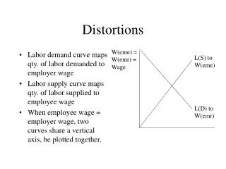
Labor demand curve maps qty. of labor demanded to employer wage Labor supply curve maps qty. of labor supplied to employee wage When employee wage = employer wage, two curves share a vertical axis, be plotted together. Distortions W(eme) = W(emr) = Wage L(S) to W(eme) L(D) to W(emr)

Distortions
E N D
Presentation Transcript
Labor demand curve maps qty. of labor demanded to employer wage Labor supply curve maps qty. of labor supplied to employee wage When employee wage = employer wage, two curves share a vertical axis, be plotted together. Distortions W(eme) = W(emr) = Wage L(S) to W(eme) L(D) to W(emr)
When employee wage does not equal employer wage, there is a distortion in the labor market. What employers pay to acquire labor does not equal what employees get for supplying labor. Labor supply and demand curves do not share an axis, cannot be plotted together. Distortions Which wage? L(S) to W(eme) L(D) to W(emr)
Problem fixed by drafting new labor supply curve that maps quantity of labor supplied to employer wage. Find out how to convert employer wage to employer wage Convert employee wages on labor supply curve to employer wages Use converted labor supply curve to find equilibrium Distortions Which wage? L(S) to W(eme) L(D) to W(emr)
Ex.: A 10% wage tax Employer wage about 10% above employee wage. Employee wages can be converted to employer wages by simply moving up the graph by about 10% Labor supply curve that maps employee wage can be converted to one that maps employer wage by moving it up graph by 10% Distortions L(S) to W(emr) Which wage? L(S) to W(eme) 10% L(D) to W(emr)
Ex.: A 10% wage tax We now have curves that tell us what L(S) and L(D) is at each employer wage. We know the employer wage where L(S) = L(D): equilibrium employer wage. Since employer wage about 10% greater than employee wage, equilibrium employee wage about 10% less than equilibrium employer wage. Distortions L(S) to W(emr) Employer wage L(S) to W(eme) 10% W(emr)* 10% W(eme)* L(D) to W(emr) L(S) = L(D) = L*
Ex.: A 10% wage tax Employer surplus (blue) equals the area above the equilibrium employer wage and below the labor demand curve. Employee surplus (green) equals the area below the equilibrium employee wage and above the old, employee-wage labor supply curve. Distortions L(S) to W(emr) Employer wage L(S) to W(eme) 10% W(emr)* 10% W(eme)* L(D) to W(emr) L(S) = L(D) = L*
Without tax: Find equilibrium using old L(S), L(D) curves Equilibrium employer wage is lower Equilibrium employee wage is higher Equilibrium quantity of labor transacted is greater Employer surplus greater Employee surplus greater Distortions L(S) to W(emr) Employer wage L(S) to W(eme) W(emr)* W(no tax)* W(eme)* L(D) to W(emr) L* L*(no tax)
Ex.: A 10% wage tax Total surplus is lower because of tax Some of lost total surplus made up by government revenue from tax collections (yellow) Some of lost total surplus is not (red), called “dead weight loss” Distortions L(S) to W(emr) Employer wage L(S) to W(eme) W(emr)* W(no tax)* W(eme)* L(D) to W(emr) L* L*(no tax)
Ex.: A 10% wage tax Total surplus is lower because of tax Some of lost total surplus made up by government revenue from tax collections (yellow) Some of lost total surplus is not (red), called “dead weight loss” Distortions L(S) to W(emr) Employer wage L(S) to W(eme) W(emr)* W(no tax)* W(eme)* L(D) to W(emr) L* L*(no tax)
Elasticity of labor demand measures sensitivity of qty. of labor demanded to employer wage. If employers reduce hiring by a lot when wage they must pay increases, then labor demand is elastic. If employers reduce hiring by only a little, then labor demand is inelastic. The Elasticity of Labor Demand W(emp) L(D) L(D) L(D) elastic W(emp) L(D) L(D) L(D) inelastic
The larger the scale and substitution effects, the greater the elasticity If increase in wage results in large increase in firms’ production costs, then firms will reduce hiring by a lot. If increase in wage results in firms substituting other kinds of labor or capital to do same work, then firms will reduce hiring by a lot. The Elasticity of Labor Demand W(emp) L(D) L(D) L(D) elastic W(emp) L(D) L(D) L(D) inelastic
A famous result about the determinants of the elasticity of labor demand are the Hicks-Marshall conditions of derived demand. Alfred Marshall, Principles of Economics (1890) John Hicks, The Theory of Wages (1943) The Hicks-Marshall Conditions W(emp) L(D) L(D) L(D) elastic W(emp) L(D) L(D) L(D) inelastic
1. The more substitutable the labor, the greater the elasticity of labor demand. If employee wage increases, firms have option of hiring substitute kinds of labor, capital, etc. The easier substitution will be, the more likely firms will do it, the greater the reduction in firms hiring. The Hicks-Marshall Conditions W(emp) L(D) L(D) L(D) elastic W(emp) L(D) L(D) L(D) inelastic
Ex.: Suppose the wages of union workers increase. Employers may say: “The union guys are great, there’s no substitute for them, I’ll still hire them, they’re worth it.” L(D) is inelastic. Or: “Why should I pay that much more for union guys? The nonunion guys are just as good. I’m switching to them.” L(D) is elastic. The Hicks-Marshall Conditions W(emp) L(D) L(D) L(D) elastic W(emp) L(D) L(D) L(D) inelastic
2. The greater the supply elasticity of substitutes, the greater the elasticity of labor demand. Increase in wage increases demand for substitutes Increase in demand bids up wage/price of substitutes, reduces substitutes’ appeal Greater substitute supply elasticity, smaller the effect The Hicks-Marshall Conditions W(emp) L(D) L(D) L(D) elastic W(emp) L(D) L(D) L(D) inelastic
2. Ex.: Suppose the wages of union workers increase. Firms subst. nonunioners Demand for nonunion workers increases. Small elasticity of labor supply of nonunion workers = increase in demand vastly bids up nonunion wage Nonunion less appealing, union workers still hired, L(D) inelastic. The Hicks-Marshall Conditions W(emp) L(D) L(D) L(D) elastic W(emp) L(D) L(D) L(D) inelastic
2. Ex.: Suppose the wages of union workers increase. Firms subst. nonunioners Demand for nonunion workers increases. Large elasticity of labor supply of nonunion workers = increase in demand hardly bids up nonunion wage Nonunion still appealing substitute, union workers get cut, L(D) elastic*. The Hicks-Marshall Conditions W(emp) L(D) L(D) L(D) elastic W(emp) L(D) L(D) L(D) inelastic
3. The greater the share of firms’ total costs paid to kind of labor, the greater elasticity of labor demand. Greater the share of costs, greater the increase in firms’ total costs caused by wage increase. Greater the increase in prices, greater decrease* in sales, greater decrease in need for all kinds of labor. The Hicks-Marshall Conditions W(emp) L(D) L(D) L(D) elastic W(emp) L(D) L(D) L(D) inelastic
3. Ex.: Suppose the wages of union workers increase. If cost of hiring union workers only 1% of total cost, then firms’ total production cost increases by only a little. Firms increase their prices by only a little, lose few customers, barely decrease production, let few union workers go. L(D) inelastic. The Hicks-Marshall Conditions W(emp) L(D) L(D) L(D) elastic W(emp) L(D) L(D) L(D) inelastic
3. Ex.: Suppose the wages of union workers increase. If cost of hiring union workers is 100% of total cost, then firms’ total production cost increases by a lot. Firms increase their prices a lot, lose many customers, seriously cut production, let many union workers go. L(D) elastic. The Hicks-Marshall Conditions W(emp) L(D) L(D) L(D) elastic W(emp) L(D) L(D) L(D) inelastic
4. The greater the product demand elasticity, the greater the elasticity of labor demand. Increase in wage increases firms’ total costs, prices Greater product demand elasticity, greater sales drop caused by price increase Greater sales drop, greater decrease in need for labor. The Hicks-Marshall Conditions W(emp) L(D) L(D) L(D) elastic W(emp) L(D) L(D) L(D) inelastic
4. Ex.: Suppose the wages of union workers increase. Increase in wage increases firms’ total costs, prices If product demand elasticity is slight, then people gladly pay higher prices, do not buy fewer goods. Firms still need as many workers as before, do not cut workers. L(D) inelastic. The Hicks-Marshall Conditions W(emp) L(D) L(D) L(D) elastic W(emp) L(D) L(D) L(D) inelastic
4. Ex.: Suppose the wages of union workers increase. Increase in wage increases firms’ total costs, prices If product demand elasticity is great, then people unwilling to pay higher prices, buy fewer goods. Firms don’t need as many workers as before, cut workers. L(D) elastic. The Hicks-Marshall Conditions W(emp) L(D) L(D) L(D) elastic W(emp) L(D) L(D) L(D) inelastic
Conditions 1-2 deal with substitution effect, 3-4 deal with scale effect. Conditions 1, 2, and 4 theoretically hold under standard economic assumptions, 3 requires more restrictive assumptions. The Hicks-Marshall Conditions W(emp) L(D) L(D) L(D) elastic W(emp) L(D) L(D) L(D) inelastic