Efficient Parallel Algorithms for Sorting and Matrix Operations

1. Lecture 24: Parallel Algorithms I • Topics: sort and matrix algorithms

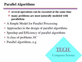
2. Processor Model • High communication latencies  pursue coarse-grain • parallelism (the focus of the course so far) • For upcoming lectures, focus on fine-grain parallelism • VLSI improvements  enough transistors to accommodate • numerous processing units on a chip and (relatively) low • communication latencies • Consider a special-purpose processor with thousands of • processing units, each with small-bit ALUs and limited • register storage

3. Sorting on a Linear Array • Each processor has bidirectional links to its neighbors • All processors share a single clock (asynchronous designs • will require minor modifications) • At each clock, processors receive inputs from neighbors, • perform computations, generate output for neighbors, and • update local storage input output

4. Control at Each Processor • Each processor stores the minimum number it has seen • Initial value in storage and on network is “*”, which is • bigger than any input and also means “no signal” • On receiving number Y from left neighbor, the processor • keeps the smaller of Y and current storage Z, and passes • the larger to the right neighbor

5. Sorting Example

6. Result Output • The output process begins when a processor receives • a non-*, followed by a “*” • Each processor forwards its storage to its left neighbor • and subsequent data it receives from right neighbors • How many steps does it take to sort N numbers? • What is the speedup and efficiency?

7. Output Example

8. Bit Model • The bit model affords a more precise measure of • complexity – we will now assume that each processor • can only operate on a bit at a time • To compare N k-bit words, you may now need an N x k • 2-d array of bit processors

9. Comparison Strategies • Strategy 1: Bits travel horizontally, keep/swap signals • travel vertically – after at most 2k steps, each processor • knows which number must be moved to the right – 2kN • steps in the worst case • Strategy 2: Use a tree to communicate information on • which number is greater – after 2logk steps, each processor • knows which number must be moved to the right – 2Nlogk • steps • Can we do better?

10. Strategy 2: Column of Trees

11. Pipelined Comparison Input numbers: 3 4 2 0 1 0 1 0 1 1 0 0

12. Complexity • How long does it take to sort N k-bit numbers? • (2N – 1) + (k – 1) + N (for output) • (With a 2d array of processors) Can we do even better? • How do we prove optimality?

13. Lower Bounds • Input/Output bandwidth: Nk bits are being input/output • with k pins – requires W(N) time • Diameter: the comparison at processor (1,1) influences • the value of the bit stored at processor (N,k) – for • example, N-1 numbers are 011..1 and the last number is • either 00…0 or 10…0 – it takes at least N+k-2 steps for • information to travel across the diameter • Bisection width: if processors in one half require the • results computed by the other half, the bisection bandwidth • imposes a minimum completion time

14. Counter Example • N 1-bit numbers that need to be sorted with a binary tree • Since bisection bandwidth is 2 and each number may be • in the wrong half, will any algorithm take at least N/2 steps?

15. Counting Algorithm • It takes O(logN) time for each intermediate node to add • the contents in the subtree and forward the result to the • parent, one bit at a time • After the root has computed the number of 1’s, this • number is communicated to the leaves – the leaves • accordingly set their output to 0 or 1 • Each half only needs to know the number of 1’s in the • other half (logN-1 bits) – therefore, the algorithm takes • W(logN) time • Careful when estimating lower bounds!

16. Matrix Algorithms • Consider matrix-vector multiplication: • yi = Sj aijxj • The sequential algorithm takes 2N2 – N operations • With an N-cell linear array, can we implement • matrix-vector multiplication in O(N) time?

17. Matrix Vector Multiplication Number of steps = ?

18. Matrix Vector Multiplication Number of steps = 2N – 1

19. Matrix-Matrix Multiplication Number of time steps = ?

20. Matrix-Matrix Multiplication Number of time steps = 3N – 2

21. Complexity • The algorithm implementations on the linear arrays have • speedups that are linear in the number of processors – an • efficiency of O(1) • It is possible to improve these algorithms by a constant • factor, for example, by inputting values directly to each • processor in the first step and providing wraparound edges • (N time steps)

22. Solving Systems of Equations • Given an N x N lower triangular matrix A and an N-vector • b, solve for x, where Ax = b (assume solution exists) • a11x1 = b1 • a21x1 + a22x2 = b2 , and so on…

23. Equation Solver

24. Equation Solver Example • When an x, b, and a meet at a cell, ax is subtracted from b • When b and a meet at cell 1, b is divided by a to become x

25. Complexity • Time steps = 2N – 1 • Speedup = O(N), efficiency = O(1) • Note that half the processors are idle every time step – • can improve efficiency by solving two interleaved • equation systems simultaneously

26. Title • Bullet