Parallel Graph Algorithms
Parallel Graph Algorithms. Aydın Buluç ABuluc@lbl.gov Lawrence Berkeley National Laboratory. CS267, Spring 2012 April 10, 2012. Some slides from: Kamesh Madduri , John Gilbert, Daniel Delling. Graph Preliminaries. n=|V| (number of vertices) m=|E| (number of edges)


Parallel Graph Algorithms
E N D
Presentation Transcript
Parallel Graph Algorithms Aydın Buluç ABuluc@lbl.gov Lawrence Berkeley National Laboratory CS267, Spring 2012 April 10, 2012 Some slides from: KameshMadduri, John Gilbert, Daniel Delling
Graph Preliminaries n=|V| (number of vertices) m=|E| (number of edges) D=diameter (max #hops between any pair of vertices) • Edges can be directed or undirected, weighted or not. • They can even have attributes (i.e. semantic graphs) • Sequences of edges <u1,u2>, <u2,u3>, … ,<un-1,un> is a path from u1 to un. Its length is the sum of its weights. • Define: GraphG = (V,E) • a set of vertices and a set of edgesbetween vertices Vertex Edge
Lecture Outline • Applications • Designing parallel graph algorithms • Case studies: • Graph traversals: Breadth-first search • Shortest Paths: Delta-stepping, PHAST • Ranking: Betweenness centrality, PageRank • Maximal Independent Sets: Luby’s algorithm • Strongly Connected Components • Wrap-up: challenges on current systems
Lecture Outline • Applications • Designing parallel graph algorithms • Case studies: • Graph traversals: Breadth-first search • Shortest Paths: Delta-stepping, PHAST • Ranking: Betweenness centrality, PageRank • Maximal Independent Sets: Luby’s algorithm • Strongly Connected Components • Wrap-up: challenges on current systems
Routing in transportation networks Road networks, Point-to-point shortest paths: 15 seconds (naïve) 10 microseconds H. Bast et al., “Fast Routing in Road Networks with Transit Nodes”,Science 27, 2007.
Internet and the WWW • The world-wide web can be represented as a directed graph • Web search and crawl: traversal • Link analysis, ranking: Page rank and HITS • Document classification and clustering • Internet topologies (router networks) are naturally modeled as graphs
3 7 1 6 8 4 10 9 2 5 Scientific Computing • Reorderings for sparse solvers • Fill reducing orderings • Partitioning, eigenvectors • Heavy diagonal to reduce pivoting (matching) • Data structures for efficient exploitation of sparsity • Derivative computations for optimization • graph colorings, spanning trees • Preconditioning • Incomplete Factorizations • Partitioning for domain decomposition • Graph techniques in algebraic multigrid • Independent sets, matchings, etc. • Support Theory • Spanning trees & graph embedding techniques Image source: YifanHu, “A gallery of large graphs” G+(A)[chordal] B. Hendrickson, “Graphs and HPC: Lessons for Future Architectures”,http://www.er.doe.gov/ascr/ascac/Meetings/Oct08/Hendrickson%20ASCAC.pdf
Large-scale data analysis • Graph abstractions are very useful to analyze complex data sets. • Sources of data: petascale simulations, experimental devices, the Internet, sensor networks • Challenges: data size, heterogeneity, uncertainty, data quality Social Informatics:new analytics challenges, data uncertainty Astrophysics: massive datasets, temporal variations Bioinformatics: data quality, heterogeneity Image sources: (1) http://physics.nmt.edu/images/astro/hst_starfield.jpg (2,3) www.visualComplexity.com
Graph –theoretic problems in social networks • Targeted advertising: clustering and centrality • Studying the spread of information Image Source: Nexus (Facebookapplication)
Network Analysis for Intelligence and Survelliance • [Krebs ’04] Post 9/11 Terrorist Network Analysis from public domain information • Plot masterminds correctly identified from interaction patterns: centrality • A global view of entities is often more insightful • Detect anomalous activities by exact/approximate subgraph isomorphism. Image Source: http://www.orgnet.com/hijackers.html Image Source: T. Coffman, S. Greenblatt, S. Marcus, Graph-based technologies for intelligence analysis, CACM, 47 (3, March 2004): pp 45-47
Research in Parallel Graph Algorithms Graph Algorithms Application Areas Methods/ Problems Architectures GPUs, FPGAs x86 multicore servers Massively multithreaded architectures (Cray XMT, Sun Niagara) Multicore clusters (NERSC Hopper) Clouds (Amazon EC2) Traversal Shortest Paths Connectivity Max Flow … … … Social Network Analysis WWW Computational Biology Scientific Computing Engineering Find central entities Community detection Network dynamics Data size Marketing Social Search Gene regulation Metabolic pathways Genomics Problem Complexity Graph partitioning Matching Coloring VLSI CAD Route planning
Characterizing Graph-theoretic computations Factors that influence choice of algorithm Input data Graph kernel • graph sparsity (m/n ratio) • static/dynamic nature • weighted/unweighted,weight distribution • vertex degree distribution • directed/undirected • simple/multi/hyper graph • problem size • granularity of computation at nodes/edges • domain-specific characteristics • traversal • shortest path algorithms • flow algorithms • spanning tree algorithms • topological sort • ….. Problem: Find *** • paths • clusters • partitions • matchings • patterns • orderings Graph problems are often recast as sparse linear algebra (e.g., partitioning) or linear programming (e.g., matching) computations
Lecture Outline • Applications • Designing parallel graph algorithms • Case studies: • Graph traversals: Breadth-first search • Shortest Paths: Delta-stepping, PHAST • Ranking: Betweenness centrality, PageRank • Maximal Independent Sets: Luby’s algorithm • Strongly Connected Components • Wrap-up: challenges on current systems
The PRAM model • Many PRAM graph algorithms in 1980s. • Idealized parallel shared memory system model • Unbounded number of synchronous processors; no synchronization, communication cost; no parallel overhead • EREW (Exclusive Read Exclusive Write), CREW (Concurrent Read Exclusive Write) • Measuring performance: space and time complexity; total number of operations (work)
PRAM Pros and Cons • Pros • Simple and clean semantics. • The majority of theoretical parallel algorithms are designed using the PRAM model. • Independent of the communication network topology. • Cons • Not realistic, too powerful communication model. • Communication costs are ignored. • Synchronized processors. • No local memory. • Big-O notation is often misleading.
Building blocks of classical PRAM graph algorithms • Prefix sums • Symmetry breaking • Pointer jumping • List ranking • Euler tours • Vertex collapse • Tree contraction [some covered in the “Tricks with Trees” lecture]
Work / Span Model tp= execution time on p processors
Work / Span Model tp= execution time on p processors t1=work
Work / Span Model tp = execution time on p processors t1 =work t∞ = span * * Also called critical-path length or computational depth.
Work / Span Model tp = execution time on p processors t1 = work t∞= span * • WORK LAW • tp≥t1/p • SPAN LAW • tp ≥ t∞ * Also called critical-path length or computational depth.
Data structures: graph representation Static case • Dense graphs (m = Θ(n2)): adjacency matrix commonly used. • Sparse graphs: adjacency lists, compressed sparse matrices Dynamic • representation depends on common-case query • Edge insertions or deletions? Vertex insertions or deletions? Edge weight updates? • Graph update rate • Queries: connectivity, paths, flow, etc. • Optimizing for locality a key design consideration.
Graph representations Compressed sparse rows (CSR) = cache-efficient adjacency lists 7 3 2 2 4 1 14 19 12 26 7 1 12 14 4 2 1 2 3 19 26 3 4 Index into adjacency array (row pointers in CSR) (column ids in CSR) Adjacencies (numerical values in CSR) Weights
Distributed graph representations • Each processor stores the entire graph (“full replication”) • Each processor stores n/p vertices and all adjacencies out of these vertices (“1D partitioning”) • How to create these “p” vertex partitions? • Graph partitioning algorithms: recursively optimize for conductance (edge cut/size of smaller partition) • Randomly shuffling the vertex identifiers ensures that edge count/processor are roughly the same
2D checkerboard distribution • Consider a logical 2D processor grid (pr * pc = p) and the matrix representation of the graph • Assign each processor a sub-matrix (i.e, the edges within the sub-matrix) 9 vertices, 9 processors, 3x3 processor grid 5 8 1 0 7 3 4 6 Flatten Sparse matrices 2 Per-processor local graph representation
High-performance graph algorithms • Implementations are typically array-based for performance (e.g. CSR representation). • Concurrency = minimize synchronization (span) • Where is the data? Find the distribution that minimizes inter-processor communication. • Memory access patterns • Regularize them (spatial locality) • Minimize DRAM traffic (temporal locality) • Work-efficiency • Is (Parallel time) * (# of processors) = (Serial work)?
Lecture Outline • Applications • Designing parallel graph algorithms • Case studies: • Graph traversals: Breadth-first search • Shortest Paths: Delta-stepping, PHAST • Ranking: Betweenness centrality, PageRank • Maximal Independent Sets: Luby’s algorithm • Strongly Connected Components • Wrap-up: challenges on current systems
Graph traversal: Depth-first search (DFS) 9 7 preorder vertex number 5 8 6 1 3 8 4 5 2 0 7 3 4 6 9 source vertex 1 2 Parallelizing DFS is a bad idea: span(DFS) = O(n) J.H. Reif, Depth-first search is inherently sequential. Inform. Process. Lett. 20 (1985) 229-234.
Graph traversal : Breadth-first search (BFS) 1 2 distance from source vertex Input: Output: 5 8 4 1 3 1 3 4 2 0 7 3 4 6 9 source vertex 1 2 • Memory requirements (# of machine words): • Sparse graph representation: m+n • Stack of visited vertices: n • Distance array: n
Parallel BFS Strategies 5 8 1. Expand current frontier (level-synchronous approach, suited for low diameter graphs) 1 • O(D) parallel steps • Adjacencies of all vertices • in current frontier are • visited in parallel 0 7 3 4 6 9 source vertex 2 2. Stitch multiple concurrent traversals (Ullman-Yannakakis approach, suited for high-diameter graphs) 5 8 • path-limited searches from “super vertices” • APSP between “super vertices” 1 source vertex 0 7 3 4 6 9 2
A deeper dive into the “level synchronous” strategy Locality (where are the random accesses originating from?) 1. Ordering of vertices in the “current frontier” array, i.e., accesses to adjacency indexing array, cumulative accesses O(n). 2. Ordering of adjacency list of each vertex, cumulative O(m). 3. Sifting through adjacencies to check whether visited or not, cumulative accesses O(m). 84 53 93 31 0 44 74 63 11 26 1. Access Pattern: idx array -- 53, 31, 74, 26 2,3. Access Pattern: d array -- 0, 84, 0, 84, 93, 44, 63, 0, 0, 11
Performance Observations Flickr social network Youtube social network Edge filtering Graph expansion
Improving locality: Vertex relabeling x x x x x x x x x x x x x • Well-studied problem, slight differences in problem formulations • Linear algebra: sparse matrix column reordering to reduce bandwidth, reveal dense blocks. • Databases/data mining: reordering bitmap indices for better compression; permuting vertices of WWW snapshots, online social networks for compression • NP-hard problem, several known heuristics • We require fast, linear-work approaches • Existing ones: BFS or DFS-based, Cuthill-McKee, Reverse Cuthill-McKee, exploit overlap in adjacency lists, dimensionality reduction x x x x x x x x x x x x x x x x x x x x x x x x x x x x x x x x x x x
Improving locality: Optimizations • Recall: Potential O(m) non-contiguous memory references in edge traversal (to check if vertex is visited). • e.g., access order: 53, 31, 31, 26, 74, 84, 0, … • Objective: Reduce TLB misses, private cache misses, exploit shared cache. • Optimizations: • Sort the adjacency lists of each vertex – helps order memory accesses, reduce TLB misses. • Permute vertex labels – enhance spatial locality. • Cache-blocked edge visits – exploit temporal locality. 84 53 93 31 0 44 74 63 11 26
Improving locality: Cache blocking Metadata denoting blocking pattern Process high-degree vertices separately Adjacencies (d) Adjacencies (d) • Instead of processing adjacencies of each vertex serially, exploit sorted adjacency list structure w/ blocked accesses • Requires multiple passes through the frontier array, tuning for optimal block size. • Note: frontier array size may be O(n) 3 2 1 x x x x x x x x x x x x x x x x x x x x x x x x frontier frontier x x Tune to L2 cache size x x x x x x x x x x x x Cache-blocked approach linear processing
Parallel performance (Orkut graph) Execution time: 0.28 seconds (8 threads) Parallel speedup: 4.9 Speedup over baseline: 2.9 Graph: 3.07 million vertices, 220 million edges Single socket of Intel Xeon 5560 (Core i7)
Graph 500 “Search” Benchmark (graph500.org) • BFS (from a single vertex) on a static, undirected R-MAT network with average vertex degree 16. • Evaluation criteria: highest performance rate (edges traversed per second) achieved on a system. • Reference MPI, shared memory implementations provided. • NERSC Hopper system is ranked #2 on current list (Nov 2011). • Over 100 billion edges traversed per second
2 • 1 • 4 • 5 • 7 • 6 • 3 Breadth-first search in the language of linear algebra • from • 1 • 7 • 1 • to • 7 • AT
2 • 1 • 4 • 5 • 7 • 6 • 3 Replace scalar operations Multiply -> select Add -> minimum • from • 1 • 7 • 1 1 1 • • to 1 1 parents: 1 • 7 • AT • X • ATX
2 • 1 • 4 • 5 • 7 • 6 • 3 Select vertex with minimum label as parent • from • 1 • 7 • 1 2 4 4 • • to 4 1 2 4 2 parents: 1 • 7 2 2 2 4 • AT • X • ATX 2
2 • 1 • 4 • 5 • 7 • 6 • 3 • from • 1 • 7 • 1 3 • • to 1 5 4 parents: 1 3 3 5 • 7 7 2 • AT • X • ATX 3 2
2 • 1 • 4 • 5 • 7 • 6 • 3 • from • 1 • 7 • 1 • • to • 7 • AT • X • ATX 6
1D Parallel BFS algorithm 2 1 ALGORITHM: • Find owners of the current frontier’s adjacency [computation] • Exchange adjacencies via all-to-all. [communication] • Update distances/parents for unvisited vertices. [computation] x 4 5 7 6 3 AT frontier x
2D Parallel BFS algorithm 2 1 x 4 5 7 6 3 AT frontier x ALGORITHM: • Gather vertices in processor column[communication] • Find owners of the current frontier’s adjacency [computation] • Exchange adjacencies in processor row [communication] • Update distances/parents for unvisited vertices. [computation]
BFS Strong Scaling • NERSC Hopper (Cray XE6, Gemini interconnect AMD Magny-Cours) • Hybrid: In-node 6-way OpenMP multithreading • Graph500 (R-MAT): 4 billion vertices and 64 billion edges. A. Buluç, K. Madduri. Parallel breadth-first search on distributed memory systems. Proc. Supercomputing, 2011.
Lecture Outline • Applications • Designing parallel graph algorithms • Case studies: • Graph traversals: Breadth-first search • Shortest Paths: Delta-stepping, PHAST • Ranking: Betweenness centrality, PageRank • Maximal Independent Sets: Luby’s algorithm • Strongly Connected Components • Wrap-up: challenges on current systems
Parallel Single-source Shortest Paths (SSSP) algorithms • Famous serial algorithms: • Bellman-Ford : label correcting - works on any graph • Dijkstra: label setting – requires nonnegative edge weights • No known PRAM algorithm that runs in sub-linear time and O(m+n log n) work • Ullman-Yannakakis randomized approach • Meyer and Sanders, ∆ - stepping algorithm • Distributed memory implementations based on graph partitioning • Heuristics for load balancing and termination detection K. Madduri, D.A. Bader, J.W. Berry, and J.R. Crobak, “An Experimental Study of A Parallel Shortest Path Algorithm for Solving Large-Scale Graph Instances,” Workshop on Algorithm Engineering and Experiments (ALENEX), New Orleans, LA, January 6, 2007.
∆ - stepping algorithm • Label-correcting algorithm: Can relax edges from unsettled vertices also • “approximate bucket implementation of Dijkstra” • For random edge weighs [0,1], runs in where L = max distance from source to any node • Vertices are ordered using buckets of width ∆ • Each bucket may be processed in parallel ∆ < min w(e) : Degenerates into Dijkstra ∆ > max w(e) : Degenerates into Bellman-Ford U. Meyer and P.Sanders, ∆ - stepping: a parallelizable shortest path algorithm. Journal of Algorithms 49 (2003)
∆ - stepping algorithm: illustration ∆ = 0.1 (say) 0.05 • One parallel phase • while (bucket is non-empty) • Inspect light (w < ∆) edges • Construct a set of “requests” (R) • Clear the current bucket • Remember deleted vertices (S) • Relax request pairs in R • Relax heavy request pairs (from S) • Go on to the next bucket 0.56 3 6 0.07 0.01 0.15 0.23 4 2 0 0.02 0.13 0.18 5 1 d array 0 1 2 3 4 5 6 ∞ ∞ ∞ ∞ ∞ ∞ ∞ Buckets
∆ - stepping algorithm: illustration 0.05 • One parallel phase • while (bucket is non-empty) • Inspect light (w < ∆) edges • Construct a set of “requests” (R) • Clear the current bucket • Remember deleted vertices (S) • Relax request pairs in R • Relax heavy request pairs (from S) • Go on to the next bucket 0.56 3 6 0.07 0.01 0.15 0.23 4 2 0 0.02 0.13 0.18 5 1 d array 0 1 2 3 4 5 6 ∞ ∞ ∞ ∞ ∞ ∞ 0 Buckets Initialization: Insert s into bucket, d(s) = 0 0 0
∆ - stepping algorithm: illustration • One parallel phase • while (bucket is non-empty) • Inspect light (w < ∆) edges • Construct a set of “requests” (R) • Clear the current bucket • Remember deleted vertices (S) • Relax request pairs in R • Relax heavy request pairs (from S) • Go on to the next bucket 0.05 0.56 3 6 0.07 0.01 0.15 0.23 4 2 0 0.02 0.13 0.18 5 1 d array 0 1 2 3 4 5 6 ∞ ∞ ∞ ∞ ∞ ∞ 0 R 2 Buckets 0 0 .01 S