Parallel Graph Algorithms
This article provides insights into parallelizing Prim's Algorithm for Minimum Spanning Tree and Dijkstra’s Algorithm for Single-Source Shortest Path. It discusses techniques for optimizing the parallel execution to achieve faster computation and better efficiency. Additionally, it explores the complexities involved in parallelizing these algorithms, including the communication and computation overhead. Practical examples and patterns are presented to demonstrate the parallel implementation of these classical graph algorithms.

Parallel Graph Algorithms
E N D
Presentation Transcript
Graph Algorithms • Minimum Spanning Tree (Prim’s Algorithm) • Single-Source Shortest Path (Dijkstra’s Algorithm) • All-Pairs Shortest Paths (Dijkstra’s and Floyd’s Algorithm)
Adjacency Matrix • An adjacency matrix represent the edges of a graph
Adjacency Matrix • Example 0 1 2 1 2 4 3 3 4 2
Prim’s Algorithm for Minimum Spanning Tree V – set of vertices VT – set of vertices in the MST E – set of edges A – adjacency matrix r – root node d – minimum distance from MST to any vertex Prim_MST(V, E, A, r) { VT = {r}; d[r] = 0; for all v in (V – VT) d[v] = Ar,v; while (VT != V) { Find a vertex u such that d[u] = min(d[v] for all v in (V – VT)); VT = VT + {u}; for all v in (V – VT) { d[v] = min(d[v], Au,v); } } } Complexity = O(n2)
Root is node b(Prim’s) a 3 Initialize 1 f 3 b 5 c 5 1 2 1 d e 4 Since d[3] = 1, add the edge b to d and consider node d next
Next consider node d(Prim’s) a 3 Take Minimums except for b and d 1 f 3 b 5 c 5 1 2 1 d e 4 Since d[0] = 1, add the edge b to a and consider node a next
Next consider node a (Prim’s) a 3 1 f 3 b 5 c 5 1 2 1 d e 4 Since d[2] = 2, add the edge d to c and consider node c next
Next consider node c(Prim’s) a 3 1 f 3 b 5 c 5 1 2 1 d e 4 Since d[4] = 1, add the edge c to e and consider node e next
Next consider node e(Prim’s) a 3 1 f 3 b 5 c 5 1 2 1 d e 4 Since d[5] = 3, add the edge a to f and consider node f next
Next consider node f(Prim’s) a 3 1 f 3 b 5 c 5 1 2 1 d e 4 VT= V so stop
Parallelizing Prim’s Algorithm • We can’t just simply execute the while loop in parallel because the d[] array changes with each selection of a vertex • We have to update values in d[] from all processors after each iteration • Suppose we have n vertices in the graph and p processors
Parallelizing Prim’s Algorithm • Partition and adjacency matrix and the distance array (d) across processors d[ ] n A 0 1 2 p-1
Parallelizing Prim’s Algorithm • Each processor computes the next vertex from among its vertices • A reduction is done on the distance array (d) to find the minimum • The result is broadcast out to all the processors
Prim’s Algorithm (Parallel) Prim_MST(V, E, A, r) { ... // Initialize d as before #pragma paraguin begin_parallel while (VT != V) { Find a vertex u such that d[u] = min(d[v] for all v in (V – VT)); VT = VT + {u}; #pragma paraguin forall for v in V if (v VT) d[v] = min(d[v], Au,v); #pragma paraguin reduce min d #pragma paraguin bcast d } #pragma paraguin end_parallel }
Prim’s Algorithm (Parallel) • Complexity of Parallel algorithm: • Each reduction and broadcast takes log p time, but we have to do up to n of them. Communication Computation
Dijkstra’s Algorithm for Single-Source Shortest Path • Given a source node, what is the shortest distance to each other node • The minimum spanning tree gives is this information
Dijkstra’s Algorithm V – set of vertices VT – set of vertices in the MST E – set of edges A – adjacency matrix r – root node d – minimum distance from root to any vertex Dijkstra_SP(V, E, A, r) { VT = {r}; d[r] = 0; for v in (V – VT) d[v] = Ar,v; while (VT != V) { Find a vertex v such that d[u] = min(d[v] for all v in (V – VT)); VT = VT + {u}; for v in (V – VT) d[v] = min(d[v], d[u] + Au,v); } } Complexity = O(n2) This is the only thing different
Source Node is node b(Dijkstra’s) a 3 Initialize 1 f 3 b 5 c 5 1 2 1 d e 4 Since d[3] = 1, consider node d next
Next consider node d(Dijkstra’s) a 3 1 f 3 b 5 c 5 1 2 1 d e 4 Since l[0] = 1, consider node a next
Next consider node a(Dijkstra’s) a 3 1 f 3 b 5 c 5 1 2 1 d e 4 Since l[2] = 3, consider node c next
Next consider node c(Dijkstra’s) a 3 1 f 3 b 5 c 5 1 2 1 d e 4 Since l[4] = 4, consider node e next
Next consider node e(Dijkstra’s) a 3 1 f 3 b 5 c 5 1 2 1 d e 4 Since d[5] = 4, add the edge a to f and consider node f next
Next consider node f(Dijkstra’s) a 3 1 f 3 b 5 c 5 1 2 1 d e 4 VT= V so stop
Parallelizing Dijkstra’s Algorithm • Since Dijkstra’s Algorithm and Prim’s Algorithm are essentially the same, we can parallelize them the same way: • Complexity of Parallel algorithm: • If we have n processors, this becomes: Communication Computation
All Pairs Shortest Path • Dijkstra’s Algorithm gives us the shortest path from a particular node to all the others • For All Paris Shortest Path, we want to find the shortest path between all pairs of vertices • We can apply Dijkstra’s Algorithm to every pair of vertices • Complexity = O(n3)
All Pairs using Dijkstra’s Algorithm V – set of vertices VT – set of vertices in the MST E – set of edges A – adjacency matrix r – root node d – minimum distance from root to any vertex Dijkstra_APSP(V, E, A) { for r in V { VT = {r}; d[r] = 0; for all v in (V – VT) d[v] = Ar,v; while (VT != V) { Find a vertex u such that d[u] = min(d[v] for all v in (V – VT)); VT = VT + {u}; for v in (V – VT) d[v] = min(d[v], d[u] + Au,v); } } } Complexity = O(n3)
All Pairs Shortest Path • We can parallelize the outermost loop • Each processors assumes a different node vi and computes the shortest path to all nodes • No communication if needed • Complexity is O(n3/p) • If we have n processors, complexity is O(n2) • If we have n2 processors, we can use n processors for each vertex. Complexity becomes O(nlogn)
Floyd’s Algorithm for All Pairs Shortest Path • Floyd’s Algorithm works off of this observation: • Consider a subset of V: • Let be the weight of the shortest path from vi to vj that includes one of the vertices in • If vk is not in the shortest path from vi to vj, then • Otherwise, the shortest path is
Floyd’s Algorithm for All Pairs Shortest Path • This leads to the following recurrence: • We can implement this using iteration and not recursion
All Pairs using Floyd’s Algorithm Floyd_APSP(V, E, A) { d0i,j = Ai,j for all i,j for k = 1 to n for i = 1 to n for j = 1 to n d(k)i,j = min(d(k-1)i,j , d(k-1)i,k + d(k-1)k,j ) • We don’t need n copies of the d matrix. We only need one. • In fact, we can do it with only one matrix V – set of vertices E – set of edges A – adjacency matrix Complexity = O(n3)
Partitioning of the d matrix • We divide the d matrix into p blocks of size n/√p • Each processor is responsible for n2/√p elements of the d matrix … … … …
Partitioning of the d matrix • However, we have to send data between processors k column j column k row i row
Communication Pattern … … … …
Analysis of Floyd’s Algorithm • Each processor has to send its block to all processors on the same row and column. • If we use a broadcast, then the time to communication is • The synchronization step requires • The time to compute the values for each processors is
Analysis of Floyd’s Algorithm • So the complexity for each step is: • And finally, the complexity for n steps (of the k loop) is: Communication Computation
A faster version of Floyd’s Algorithm • We can do a pipeline of values moving through the matrix. • The reason is because once processor pi, j computes the value of it can then send it to the processors pi, j-1 , pi, j+1 , pi+1, j , and pi-1, j
Consider the movement of the value computed by processor 4 Time t t+1 t+2 t+3 t+4 1 2 3 4 5 6 7 8 Processors
Analysis of Floyd’s Algorithm with pipelining • The net complexity of the algorithm using pipelining is: Communication Computation