1 p1 p2 p7 2 p3 p5 p8 3 p4 p6 p9

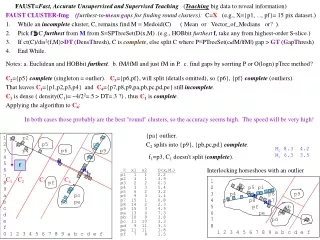
1. FAUST = Fast, Accurate Unsupervised and Supervised Teaching (Teaching a table to reveal it's information) FAUST CLUSTER (a divisive, FAUSTian clustering method) Start with one cluster, C, consisting of all points in the table, X. On each cluster, C, not yet complete: 1. Pick f to be a point in C furthest from the centroid, M (M = mean or vector_of_medians or?) 2. If density(C)≡count(C)/d(M,f)2 > DT, declare C complete, else pick g to be a point furthest from f. 3. (fission step) Replace M with two new centroids which are the points on the fg-line_segment the fraction, h, in from the endpoints, f and g. Divide C into two new clusters by assigning each point to the closest of two new centroids. Note that singleton clusters are always complete since density(singleton) = 1/0 =  > DT no matter what DT is. In our example, centriod=mean; h=1; DT= 1.5 C1 = all points closer to f=p1 than g=pe C2↓ 1 p1 p2 p7 2 p3 p5 p8 3 p4 p6 p9 4 pa 5 6 7 8 pf 9 pb a pc b pd pe c d e f 0 1 2 3 4 5 6 7 8 9 a b c d e f dist to M 8.4 6.7 7.1 5.8 3.7 1.7 7.4 6.0 6.6 4.4 4.4 5.7 6.2 6.7 3.6 dis tof(=p1) 0 2 1.41 2.82 5.09 8.24 14 13.0 14.1 12.3 12.0 13.4 12.8 14.1 9.21 dis tog(=pe) 14.1 12.8 12.7 11.3 10.2 8.24 10.7 9.48 8.94 7.28 2.23 1 2 0 5 M1 X x1 x2 p1 1 1 p2 3 1 p3 2 2 p4 3 3 p5 6 2 p6 9 3 p7 15 1 p8 14 2 p9 15 3 pa 13 4 pb 10 9 pc 11 10 pd 9 11 pe 11 11 pf 7 8 M0 M2 density(C)=16/8.42 = .23 < DT=1.5 so C is not complete M0 8.6 4.7 M1 3 1.8 M2 11 6.2

2. FAUST CLUSTER clusters C1. C11 and C12 C11: closer to p1 than p5 C12 ↓ 1 p1 p2 2 p3 p5 3 p4 4 5 6 7 8 9 a b c d e f 0 1 2 3 4 5 6 7 8 9 a b c d e f M1 dist toM11 1.4 1.0 0.3 1.4 dist to p5 5.09 3.16 4 3.16 0 dist toM1 2.1 0.8 1.0 1.2 3.0 dist top1 0 2 1.41 2.82 5.09 C1 x1 x2 p1 1 1 p2 3 1 p3 2 2 p4 3 3 p5 6 2 M1 (3 1.8) M11 (2.3 1.8) y11 = p1 C1= {p1,p2,p3,p4,p5} has density ≡ count/d(M1,f1)2 = 5/32 = 5/9 < DT, so it is not compete! (further fission required). C12 = {p5} is a singleton cluster and therefore complete (an outlier). C11 = {p1,p2,p3,p4} has density ≡ count/d(M11,f11)2 = 4/1.42 = 4/2 = 2 > DT, so compete! (no further fission). Aside: We probably would not declare the 4 points in C11 as outliers due to C11's relatively large size (4 out of a total of 16) Reminder: We assume clusters are round and that outlier-ness or anomalousness depends upon both smallness in size and largeness in separation distance.

3. FAUSTCLUSTER clusters C2, C21 and C22 C21: closer to p7 than pd C22↓ 1 p7 2 p8 3 p6 p9 4 pa 5 6 7 8 pf 9 pb a pc b pd pe c d e f 0 1 2 3 4 5 6 7 8 9 a b c d e f dist pd 8 11.6 10.2 10 8.06 2.23 2.23 0 2 3.60 dis M21 4.2 2.4 1 1.8 1.4 dis M22 0.8 1.4 1.3 1.8 3.1 M2 dist p7 6.32 0 1.41 2 3.60 9.43 9.84 11.6 10.7 10.6 dis M2 4 6.3 4.9 4.8 2.7 3.1 3.8 5.3 4.8 4.7 C2 x1 x2 p6 9 3 p7 15 1 p8 14 2 p9 15 3 pa 13 4 pb 10 9 pc 11 10 pd 9 11 pe 11 11 pf 7 8 M2 (11 6.2) M21 (13.2 2.6) M22 ( 9.6 9.8) C2= {p6,p7,p8,p9,pa,pb,pc,pe,pf} has density ≡ count/d(M2,f2)2 = 10/6.32 = .251 < DT, so it is not complete. C21 = {p6,p7,p8,p9,pa} has density =5/4.22 = .285 < DT Not dense enough so not complete. C22 = {pb,pc,pd,pe,pf} has density = 5/3.12 = .52 < DT Not dense enough so not complete.

4. FAUST CLUSTER clusters C22, C221 and C222 C221 Closer to pe than pf C222↓ 1 2 3 4 5 6 7 8 pf 9 pb a pc b pd pe c d e f 0 1 2 3 4 5 6 7 8 9 a b c d e f dist pe 2.2 1 2 0 5 dist pf 3.1 4.4 3.6 5 0 dis M22 0.8 1.4 1.3 1.8 3.1 dis M221 1.2 0.7 1.4 1.0 C22 x1 x2 pb 10 9 pc 11 10 pd 9 11 pe 11 11 pf 7 8 M22 M22 (9.6 9.8) M221 (10.2 10.2) C222 = {pf} is singleton so complete ( outlier or anomaly). C221 = {pb,pc,pd,pe} has density = 4/1.42 = 2.04 > DT, dense enough, so complete. Again, this cluster might not be declared a set of outliers since its' relative size is large.

5. FAUST CLUSTER clusters C21, C211 and C212 C211 closer to p6 than p7 C212↓ 1 p7 2 p8 3 p6 p9 4 pa 5 6 7 8 9 a b c d e f 0 1 2 3 4 5 6 7 8 9 a b c d e f M7 dist p7 6.3 0 1.4 2 3.6 dist p6 0 6.3 5.0 6 4.1 dis M7 4.2 2.4 1 1.8 1.4 dis M212 1.6 0.5 0.9 1.9 C21 x1 x2 p6 9 3 p7 15 1 p8 14 2 p9 15 3 pa 13 4 M21 (13.2 2.6) M212 (14.2 2.5) C211 = {p6} is singleton so complete. (outlier or anomaly). C212 = {p7,p8,p9,pa} has density = 4/1.92 = 1.11 < DT so not complete.

6. FAUST CLUSTER clusters C212, C2121 and C2122 C2121 closer to p7 than pa C2122↓ 1 p7 2 p8 3 p9 4 pa 5 6 7 8 9 a b c d e f 0 1 2 3 4 5 6 7 8 9 a b c d e f M212 dist p7 0 1.4 2 3.6 dist pa 3.6 2.2 2.2 0 dis M212 1.6 0.5 0.9 1.9 dis M2121 1.0 0.6 1.0 C212 x1 x2 p7 15 1 p8 14 2 p9 15 3 pa 13 4 M212 (14 2.5) M2121 (14.6 2 ) C2122 = {pa} is singleton so complete (outlier or anomaly). C2121 = {p7,p8,p9} has density = 3/12 = 3 > DT complete. From this example, can we see that using the points, say, 1/8 and 7/8 of the way from pa to p7 would make better centroids? (so that p9 would be more substantially closer to p7 than it is to pa?)

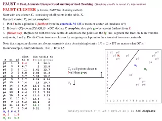
7. FAUST CLUSTER: Start with one cluster, C, consisting of all points in the table, X. On each cluster, C, not yet complete: 1. Pick f to be a point in C furthest from the centroid, M (M = mean or vector_of_medians or?) 2. If density(C)≡count(C)/d(M,f)2 > DT, declare C complete, else pick g to be a point furthest from f. 3. (fission step) Replace M with two new centroids which are the points on the fg-line_segment the fraction, h, in from the endpoints, f and g. Divide C into two new clusters by assigning each point to the closest of two new centroids. In this example, centriod=mean; h=1; DT= 1.5 There are 4 outliers and 3 non-outlier clusters. If DT=1.1 then {pa} joins {p7,p8,p9}. If DT=0.5 then in addition, {pf} joins {pb,pc.pd,pe}, {p5} joins {p1,p2,p3,p4}. 1 p1 p2 p7 2 p3 p5 p8 3 p4 p6 p9 4 pa 5 6 7 8 pf 9 pb a pc b pd pe c d e f 0 1 2 3 4 5 6 7 8 9 a b c d e f

8. MASTERMINE (Medoid-based Affinity Subset deTERMINEr) Declare {r1,r2,r3,O} mean=(8.18, 3.27, 3.73) vom=(7,4,3) dim2 11,10 4,9 2,8 5,8 4,6      3,4 6.3,5.9 6,5.5 10,5 9,4   8,3 7,2 median mean median median mean mean mean median median median mean median mean mean dim1 Alg1: Choose dim. 3 clusters, {r1,r2,r3,O}, {v1,v2,v3,v4}, {0} by: 1.a: when d(mean,median) >c*width, declare cluster. 1.b: Same alg on subclusts. Declare {0,v1} or {v1,v2}? Take {v1,v2} (on median side of mean). Makes {0} a cluster (outlier, since it's singleton). Continuing with {v1,v2}: dim2 o 0 r1 v1 r2 v2 r3 v3 v4 Declare {v1,v2,v3,v4}. Have to loop, but not on next m projs if close? Can skip doubletons since mean always same as median. Alg2: 2.a density > Density_Thresh, declare(density≡count/size). Oblique: grid of Oblique dir_vects, e.g., For 3D, DirVect from each PTM triangle. With projections onto those lines, do 1 or 2 above. Order = any sphere grid: Sn≡{x≡(x1...xn)Rn | xi2=1}, polar coords. lexicographical polar coords? 180n too many? Use e.g., 30 deg units, giving 6n vectors, for dim=n. Attrib relevance important! Alg1-2: Use 1st criteria to trigger from 1.a, 2.a to declare clusters. Alg3: Calc mean and vom. Do 1a or 1b on line connecting them. Repeat on each cluster, use another line? Adjust proj lines, stop cond dim1 Alg4: Proj to mean-vom-line, mn=6.3,5.9 vom=6,5.5 (11,10=outlier). 4.b, perp line? 3 435  524 504 545    323     924 b43      e43 c63       752            f72 1 Other option? use a p-Kmeans approach. Could use K=2 and divisive (using a GA mutation at various times to get us off a non-convergent track)? 1. no clusters determined yet. 2 Notes:Each round, reduce dim by one (low bound on the loop.) Each round, just need good line (in remaining hyperplane) to project cluster (so far). 1. pick line thru proj'd mean, vom (vom is dependent on basis used. better way?) 2. pick line thru longest diameter? ( or diam  1/2 previous diam?). 3. try a direction vector. Then hill climb it in direction increase in diam of proj'd set. 2.(9,2,4) determined as an outlier cluster. 3.Use red dim line, (7,5,2) an outlier cluster. maroon pts determined as cluster, purple pts too. 3.a use mean-vom again would the same be determined?

9. Separate class R using midpoint of means method: Calc a vomV vomR d-line d v2 v1 std of distances, vod, from origin along the d-line FAUST Oblique (our best classifier?) PR=P(X o dR ) < aR1 pass gives classR pTree D≡ mRmV d=D/|D| (mR+(mV-mR)/2)od = a = (mR+mV)/2od(works also if D=mVmR, Training≡placingcut-hyper-plane(s) (CHP) (= n-1 dim hyperplane cutting space in two). Classification is 1 horizontal program (AND/OR) across pTrees, giving a mask pTree for each entire predicted class (all unclassifieds at-a-time) Accuracy improvement? Consider the dispersion within classes when placing the CHP. E.g., use the 1. vectors_of_median, vom, to represent each class, not the meanmV, where vomV ≡(median{v1|vV}, 2. midpt_std, vom_std methods: project each class on d-line; then calculate std (one horizontal formula per class using Md's method); then use the std ratio to place CHP (No longer at the midpoint between mr and mv median{v2|vV}, ...) dim 2 Note:training (finding a and d) is a one-time process. If we don’t have training pTrees, we can use horizontal data for a,d (one time) then apply the formula to test data (as pTrees) r   r vv r mR   r v v v     r    r v mV v r v v r v dim 1

10. 1 A1,bw1 A1,bw1-1 ... A1,0 A2,bw2 ... Ak+1,c1 ..An,ccn 2 3 4 1 0 0 0 1 0 0 1 5 ... 0 1 1 0 0 1 1 2 7B 0 0 0 0 0 0 0 P 3 1 0 0 0 1 0 0 4 0 0 1 0 0 0 1 5 1 0 0 0 1 0 0 ... 0 0 1 0 0 0 0 N A1,bw1 A1,bw1-1 ... A1,0 A2,bw2 ... Ak+1,c1 ...An,ccn row number 1 0 1 0 1 1 0 1 1 1 1 0 0 0 1 2 gene chromosome 0 0 0 0 0 0 0 ... 1 0 0 0 1 0 1 roof (N/64) bpp 1 2 3 4 5 ... 3B inteval number pc bc lc cc pe age ht wt 1 0 0 0 1 0 0 0 1 1 0 0 1 1 0 0 0 0 0 0 0 1 0 0 0 1 0 0 0 0 1 0 0 0 1 1 0 0 0 1 0 0 0 0 1 0 0 0 0 AHG(P,bpp) APPENDIX: The PTreeSet Genius for Big Data Big Vertical Data: PTreeSet (Dr. G. Wettstein's) perfect for BVD! (pTrees both horiz and vert) PTreeSets incl methods for horiz querying and vertical DM, multihopQuery/DM, and XML. T(A1...An) is a PTreeSet data structure = bit matrix with (typically) each numeric attr converted to fixedpt(?), (negs?) bitsliced (pt_posschema) and category attr bitmapped; coded then bitmapped; num coded then bisliced (or as is, ie, char(25) NAME col stored outside PTreeSet? A1..Ak num w bitwidths=bw1..bwk; Ak+1..An categorical w counts=cck+1...ccn, PTreeSet is bitmatrix: Methods for this data structure can provide fast horizontal row access , e.g., an FPGA could (with zero delay) convert each bit-row back to original data row. Methods already exist to provide vertical (level-0 or raw pTree) access. Add any Level1 PTreeSet can be added: given any row partition (eg, equiwidth =64 row intervalization) and a row predicate (e.g.,  50% 1-bits ). Add "level-1 only" DM meth, e.g., FPGA converts unclassified rowsets to equiwidth=64, 50% level1 pTrees, then entire batch would be FAUST classified in one horiz program. Or lev1 pCKNN. pDGP (pTree Darn Good Protection) by permuting col ord (permution = key). Random pre-pad for each bit-column would makes it impossible to break the code by simply focusing on the first bit row. More security?: all pTrees same (max) depth, and intron-like pads randomly interspersed... Relationships (rolodex cards) are 2 PTreeSets, AHGPeoplePTreeSet (shown) and AHGBasePairPositionPTreeSet (rotation of shown). Vertical Rule Mining, Vertical Multi-hop Rule Mining and Classification/Clustering methods (viewing AHG as either a People table (cols=BPPs) or as a BPP table (cols=People). MRM and Classification done in combination? Any table is a relationship between row and column entities (heterogeneous entity) - e.g., an image = [reflect. labelled] relationship between pixel entity and wavelength interval entity. Always PTreeSetting both ways facilitates new research and make horizontal row methods (using FPGAs) instantaneous (1 pass across the row pTree) Most bioinformatics done so far is not really data mining but is more toward the database querying side. (e.g., a BLAST search). A radical approach View whole Human Genome as 4 binary relationships between People and base-pair-positions (ordered by chromosome first, then gene region?). AHG [THG/GHG/CHG] is relationship between People and adenine(A) [thymine(T)/guanine(G)/cytosine(C)] (1/0 for yes/no) Order bpp? By chromosome and by gene or region (level2 is chromosome, level1 is gene within chromosome.) Do it to facilitate cross-organism bioinformatics data mining? Create both People and BPP-PTreeSet w human health records feature table (training set for classification and multi-hop ARM.) comprehensive decomp (ordering of bpps) FOR cross species genomic DM. If separate PTreeSets for each chrmomsome (even each region - gene, intron exon...) then we can may be able to dataming horizontally across the all of these vertical pTrees. The red person features used to define classes. AHGp pTrees for data mining. We can look for similarity (near neighbors) in a particular chromosome, a particular gene sequence, of overall or anything else.

11. Facebook-Buys: A facebook Member, m, purchases Item, x, tells all friends. Let's make everyone a friend of him/her self. Each friend responds back with the Items, y, she/he bought and liked. I≡Items I≡Items I≡Items F≡Friends(M,M) Members F≡Friends(K,B) F≡Friends(K,B) Buddies Buddies 1 0 1 1 4 1 1 0 0 1 1 1 1 4 4 0 1 0 0 3 0 0 1 1 0 0 0 0 3 3 1 0 0 1 2 1 1 0 0 0 0 1 1 2 2 0 0 1 0 1 0 0 0 0 1 1 0 0 1 1 P≡Purchase(M,I) P≡Purchase(B,I) P≡Purchase(B,I) Kiddos Kiddos 2 4 4 4 2 2 3 3 3 3 3 3 2 2 4 4 2 4 1 5 5 5 1 1 Members Groupies Groupies 4 4 1 1 0 0 1 1 1 1 4 4 1 2 4 2 2 2 4 1 3 3 0 0 1 1 0 0 0 0 3 3 2 2 1 1 0 0 0 0 1 1 2 2 0 0 1 1 0 1 0 0 1 0 1 1 1 1 0 1 1 0 1 1 1 0 1 1 1 1 1 1 0 1 0 1 1 0 1 1 1 1 1 0 1 1 1 1 0 0 1 1 1 1 1 1 1 1 1 0 1 1 1 1 1 0 0 0 0 0 0 1 1 1 4 4 4 3 3 3 2 2 2 1 1 1 4 4 4 0 0 0 0 1 1 0 0 1 1 1 0 0 0 0 0 0 0 Others(G,K) Compatriots (G,K) 1 1 1 1 1 1 1 1 1 1 1 0 0 0 1 1 1 1 1 1 2 2 2 1 0 0 0 1 1 0 0 Kx=OR Ogx frequent if Kx large (tractable- one x at a time and OR. gORbPxFb XI MX≡&xXPx People that purchased everything in X. FX≡ORmMXFb = Friends of a MX person. So, X={x}, is Mx Purchases x strong" Mx=ORmPxFmx frequent if Mx large. This is a tractable calculation. Take one x at a time and do the OR. K2 = {1,2,4} P2 = {2,4} ct(K2) = 3 ct(K2&P2)/ct(K2) = 2/3 Mx=ORmPxFmx confident if Mx large. ct( Mx  Px ) / ct(Mx) > minconf To mine X, start with X={x}. If not confident then no superset is. Closure: X={x.y} for x and y forming confident rules themselves.... ct(ORmPxFm & Px)/ct(ORmPxFm)>mncnf Fcbk buddy, b, purchases x, tells friends. Friend tells all friends. Strong purchase poss? Intersect rather than union (AND rather than OR). Ad to friends of friends K2={2,4} P2={2,4} ct(K2) = 2 ct(K2&P2)/ct(K2) = 2/2 K2={1,2,3,4} P2={2,4} ct(K2) = 4 ct(K2&P2)/ct(K2)=2/4

12. The Multi-hop Closure Theorem A hop is a relationship, R, hopping from entities E to F. Lemma-2: Let AD, &clist(&aDXa)Yc covers Lemma-2: Let AD, &clist(&aDXa)Yc covers &clist(&aAXa)Yc &clist(&aAXa)Yc A'=list(&aDXa)  D'=list(&aAXa) so by lemma-1, we get lemma-2: Lemma-3: AD, &elist(&clist(&aAXa)Yc)We covers &elist(&clist(&aDXa)Yc)We A condition is downward [upward]closed: If when it is true of A, it is true for all subsets [supersets], D, of A. Given an (a+c)-hop multi-relationship, where the focus entity is a hops from the antecedent and c hops from the consequent, if a [or c] is odd/eventhendownward/upwardclosure applies to frequency and confidence. A pTree, X, is said to be "covered by" a pTree, Y, if  one-bit in X, there is a one-bit at that same position in Y. Lemma-0: For any two pTrees, X and Y, X&Y is covered by X and thus ct(X&Y)  ct(X) and list(X&Y)list(X) Proof-0: ANDing with Y may zero some of X's ones but it will never change any zeros to ones. Lemma-1: Let AD, &aAXa covers &aDXa Proof-1&2: Let Z=&aD-AXa then &aDXa =Z&(&aAXa). lemma-1 now follows from lemma-0, as does Proof-3: lemma-3 in the same way from lemma-1 and lemma-2. Continuing this establishes: If there are an odd number of nested &'s then the expression with D is covered by the expression with A. Therefore the count with D  with A. Thus, if the frequent expression and the confidence expression are > threshold for A then the same is true for D. This establishes downward closure. Exactly analogously, if there are an even number of nested &'s we get the upward closures.

13. PTM_LLRR_LLRR_LR... What ordering is best for spherical data (e.g., Astronomical bodies on the celestial sphere, sharing origin and equatorial plane with earth and no radius. Hierarchical Triangle Mesh (HTM) orders equilateral triangulations (recursively). Ptree Triangle Mesh (PTM) does also. (RA=Recession Angle; dec=declination) L L L R L R R R R L R R R R L L L L L L L L L L L L L L L L R L R R R R R R R R R R R R R R R R L R R R L L L L L 1,2 1,1,2 1,0 1,1,1 1,1 1,1,0 1,3 1.1.3 HTM sub-triangle ordering For PTM, Peel from south to north pole along quadrant great circles and the equator. 1 Level-2 follows the level-1 LLRR pattern with another LLRR pattern. Level-3 follows level-2 with LR when level-2 pattern is L and RL when level-2 pattern is R Mathematical theorem: n,  an n-sphere filling (n-1)-sphere? Corollary:  sphere filling circle (2-sphere filling 1-sphere). ... Proof-2: Let Cn ≡ the level-n circle, C ≡ limitnCn is a circle which fills the 2-sphere! Proof: Let x be any point on the 2-sphere. distance(x,Cn)  sidelength (=diameter) of the level-n triangles. sidelengthn+1 = ½ * sidelengthn. d(x,C) ≡ lim d(x,Cn)  lim sidelengthn  sidelength1 * lim ½n = 0 x See 2012_05_07 notes for level-4 circle.

14. K-means: Assign each pt to closest mean and increment sum, count for mean recalculation (1 scan). Iterate until stop_cond. pK-means: Same as above, but both assignment and means recalculation are done without scanning: 1.Pick K centroids, {Ci}i=1..K 2. Calc SPTreeSet, Di=D(X,Ci) (col of distances from all x to Ci) to get P(DiDj) i<j ( predicate is dis(x,Ci)dis(x,Cj) ). 4. Calculate the mask-pTrees for the clusters goes as follows: PC1 = P(D1D2) & P(D1D3) & P(D1D4) & ... & P(D1DK) PC2 = P(D2D3) & P(D2D4) & ... & P(D2DK) & ~PC1 PC3 = P(D3D4) & ... & P(D3DK) & ~PC1 & ~PC2 . . . PCk = & ~PC1 & ~PC2 & ... & ~PCK-1 5. Calculate new Centroids, Ci = Sum(X&PCi)/count(PCi) 6. If stop_cond=false, start next iteration with new centroids. Note: In 2. above, Md's 2's complement formulas can be used to get mask pTrees, P(DiDj) or FAUST (using Md's dot product formula) can be used. Is one faster than the other? pKl-means: ( P K-less means, pronouncedpickle means) For all K: 4'. Calculate cluster mask pTrees. For K=2..n, PC1K = P(D1D2) & P(D1D3) & P(D1D4) & ... & P(D1DK) PC2K = P(D2D3) & P(D2D4) & ... & P(D2DK) & ~PC1 . . . PCK = P(X) & ~PC1 & ... & ~PCK-1 6'. If  k s.t. stop_cond = true, stop and choose that k, else start the next iteration with these new centroids. 3.5'. Continue with certain k's only (e.g., top t? Top means? a. Sum of cluster diams (use max, min of D(Clusteri, Cj), or D(Clusteri. Clusterj) ). b. Sum of diams of cluster gaps (Use D(listPCi, Cj) or D(listPCi, listPCj). c. other? Fusion: Check for clusters that should be fused?  Fuse (decrease k) 1. Empty clusters with any other and reduce k (this is probably assumed in all k-means methods since there is no mean.). 2. For some a>1, max(D(CLUSTi,Cj))< a*D(Ci,Cj) and max(D(CLUSTj,Ci))< a*D(Ci,Cj), fuse CLUSTi and CLUSTj. Avg better? Fission: Split cluster (increase k), if a. mean and vom are quite far apart, b. cluster is sparse (i.e., max(D( CLUS,C))/count(CLUS)<T (Pick fission centroid y at max dis from C. Pick z at max dis from y. (diametric opposites in C) Sort PTreeSet(dis(x,X-x)), then sort desc, gives singleton-outlier-ness. Or take global medoid, C, increase r until  ct(dis(x,Disk(C,r)))>ct(X)–n, then declare compliment outliers. .Or, loop x once - alg is O(n). ( O(n2) for horiz: x, find dis(x,y) yx (O(n(n-1)/2)=O(n2). Or predict C so it is not X-x but a fixed subset? Or create 3 col “distance table”,  DIS(x,y,d(x,y))  (limit it to only those distances < thresh?) where dis(x,y) is a PTreeSet of those distances. If we have DIS as a PTreeSet both ways - have one for “y-pTrees” and another for “x-pTrees”. y’s --> x’s  0  2  1  3  1  2… v       0  2  5  9  1… y’s close to x are in it’s cluster.  If small, and next larger d(x,y) is large, x-cluster members are outliers.

15. Mark Silverman: I start randomly - converges in 3 cycles. Here I increase k from 3 to 5. 5th centroid could not find a member (at 0,0), 4th centroid picks up 2 points that look remarkably anomalous Treeminer, Inc. (240) 389-0750 WP: Start with large k? Each round, "tidy up" by fusing pairs of clusters using   max( P(dis(CLUSi, Cj))) < dis(Ci, Cj) and max( P(dis(CLUSj, Ci))) < dis(Ci, Cj) ? Eliminate empty clusters and reduce k. (Avg better than max ? in the above). Mark: Curious about one other state it converges to. Seems like when we exceed optimal k, some instability. WP: Tiding up would fuse Series4 and series3 into series34 Then calc centroid34. Next fuse Series34 and series1 into series134, calc centrod34 Also?: Each round, split a cluster (create 2nd centroid) if mean and vector_of_medians far apart. (A second go at this mitosis based on density of the cluster. If a cluster is too sparse, split it. A pTree (no looping) sparsity measure:   max(dis( CLUSTER,CENTROID )) / count(CLUSTER) X