Download
1 / 20
200 likes | 213 Vues
FAUST CLUSTER-fmg utilizes furthest-to-mean gaps to find round clusters in big datasets effectively and accurately without human supervision. The algorithm iteratively identifies complete and incomplete clusters based on density thresholds, splitting them accordingly to reveal valuable information. Euclidean distance and HOBbit furthest methods are employed to determine dense and sparse clusters. The process involves multiple steps and calculations to ensure high accuracy and efficiency.

E N D
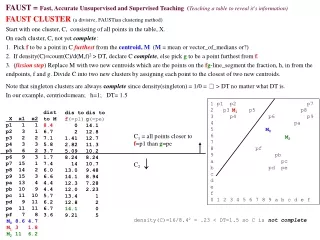
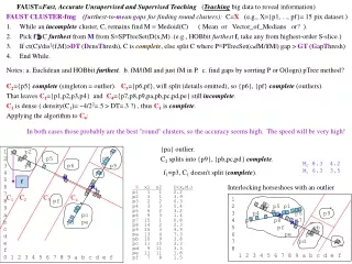
FAUST=Fast, Accurate Unsupervised and Supervised Teaching(Teachingbig data to reveal information) • FAUST CLUSTER-fmg (furthest-to-meangaps for finding round clusters):C=X (e.g., X≡{p1, ..., pf}= 15 pix dataset.) • While an incomplete cluster, C, remains find M ≡ Medoid(C) ( Mean or Vector_of_Medians or? ). • Pick fC furthest fromM from S≡SPTreeSet(D(x,M) .(e.g., HOBbit furthestf, take any from highest-order S-slice.) • If ct(C)/dis2(f,M)>DT (DensThresh), C is complete, else split C where P≡PTreeSet(cofM/|fM|) gap > GT (GapThresh) • End While. • Notes: a. Euclidean and HOBbit furthest. b. fM/|fM| and just fM in P. c. find gaps by sorrting P or O(logn) pTree method? Interlocking horseshoes with an outlier 1 2 p2 p5 p1 3 p4 p6 p9 4 p3 p8 p7 5 pf pb 6 pe pc 7 pd pa 8 1 2 3 4 5 6 7 8 9 a b c d e f C2={p5} complete (singleton = outlier). C3={p6,pf}, will split (details omitted), so {p6}, {pf} complete (outliers). That leaves C1={p1,p2,p3,p4} and C4={p7,p8,p9,pa,pb,pc,pd,pe} still incomplete. C1 is dense ( density(C1)= ~4/22=.5 > DT=.3 ?) , thus C1is complete. Applying the algorithm to C4: In both cases those probably are the best "round" clusters, so the accuracy seems high. The speed will be very high! {pa} outlier. C2 splits into {p9}, {pb,pc,pd} complete. 1 p1 p2 p7 2 p3 p5 p8 3 p4 p6 p9 4 pa 5 6 7 8 pf 9 pb a pc b pd pe c d e f 0 1 2 3 4 5 6 7 8 9 a b c d e f M0 8.3 4.2 M1 6.3 3.5 f1=p3, C1 doesn't split (complete). M f M4 X x1 x2 p1 1 1 p2 3 1 p3 2 2 p4 3 3 p5 6 2 p6 9 3 p7 15 1 p8 14 2 p9 15 3 pa 13 4 pb 10 9 pc 11 10 pd 9 11 pe 11 11 pf 7 8 D(x,M0) 2.2 3.9 6.3 5.4 3.2 1.4 0.8 2.3 4.9 7.3 3.8 3.3 3.3 1.8 1.5 C1 C2 C3 C4 M1 M0
FAUST CLUSTER-fmg:O(logn) pTree method for finding P-gaps: P ≡ ScalarPTreeSet( c ofM/|fM| ) xoUp1M 1 3 3 4 6 9 14 13 15 13 13 14 13 15 10 P3 0 0 0 0 0 1 1 1 1 1 1 1 1 1 1 P2 0 0 0 1 1 0 1 1 1 1 1 1 1 1 0 P1 0 1 1 0 1 0 1 0 1 0 0 1 0 1 1 P0 1 1 1 0 0 1 0 1 1 1 1 0 1 1 0 X x1 x2 p1 1 1 p2 3 1 p3 2 2 p4 3 3 p5 6 2 p6 9 3 p7 15 1 p8 14 2 p9 15 3 pa 13 4 pb 10 9 pc 11 10 pd 9 11 pe 11 11 pf 7 8 D(x,M) 8 7 7 6 4 2 7 6 7 4 4 6 6 7 4 D3 1 0 0 0 0 0 0 0 0 0 0 0 0 0 0 D2 0 1 1 1 1 0 1 1 1 1 1 1 1 1 1 D1 0 1 1 1 0 1 1 1 1 0 0 1 1 1 0 D0 0 1 1 0 0 0 1 0 1 0 0 0 0 1 0 HOBbit Furthest pt list ={p1} Pick f=p1. dens(C)=16/82=16/64=.25 If GT=2k then add 0,1,...,2k-1 check all k of these down to level=2k P3'=[0,7] 1 1 1 1 1 0 0 0 0 0 0 0 0 0 0 ct=5 P3=[8,15] 0 0 0 0 0 1 1 1 1 1 1 1 1 1 1 ct= 10 P3'&P2 =[4,7] 0 0 0 1 1 0 0 0 0 0 0 0 0 0 0 ct =2 P3&P2' =[8,11] 0 0 0 0 0 1 0 0 0 0 0 0 0 0 1 ct =2 P3&P2 =[12,15] 0 0 0 0 0 0 1 1 1 1 1 1 1 1 0 ct =8 P3'&P2' =[0,3] 1 1 1 0 0 0 0 0 0 0 0 0 0 0 0 ct =3 P3'&P2'&P1' =[0,1] 1 0 0 0 0 0 0 0 0 0 0 0 0 0 0 ct =1 P3&P2'&P1' =[8,9] 0 0 0 0 0 1 0 0 0 0 0 0 0 0 0 ct =1 P3&P2'& P1= [10,11] 0 0 0 0 0 0 0 0 0 0 0 0 0 0 1 ct=1 P3'&P2'&P1 =[2,3] 0 1 1 0 0 0 0 0 0 0 0 0 0 0 0 ct =2 P3'&P2&P1' =[4,5] 0 0 0 1 0 0 0 0 0 0 0 0 0 0 0 ct =1 P3'&P2&P1 =[6,7] 0 0 0 0 1 0 0 0 0 0 0 0 0 0 0 ct=1 P3&P2&P1' =[12,13] 0 0 0 0 0 0 0 1 0 1 1 0 1 0 0 ct =3 P3&P2&P1 =[14,15] 0 0 0 0 0 0 1 0 1 0 0 1 0 1 0 ct =4 0 0 0 0 0 0 0 0 0 0 0 0 0 0 0 P3'&P2' &P1'&P0' 0ct=0 1 0 0 0 0 0 0 0 0 0 0 0 0 0 0 P3'&P2' &P1'&P0 1ct=1 0 0 0 0 0 0 0 0 0 0 0 0 0 0 0 P3'&P2' &P1&P0' 2ct=0 0 1 1 0 0 0 0 0 0 0 0 0 0 0 0 P3'&P2' &P1&P0 3ct=2 0 0 0 1 0 0 0 0 0 0 0 0 0 0 0 P3'&P2& P1'&P0' 4ct=0 0 0 0 0 0 0 0 0 0 0 0 0 0 0 0 P3'&P2 &P1'&P0 5ct=0 0 0 0 0 1 0 0 0 0 0 0 0 0 0 0 P3'&P2& P1&P0' 6ct=1 0 0 0 0 0 0 0 0 0 0 0 0 0 0 0 P3'&P2 &P1&P0 7ct=0 0 0 0 0 0 0 0 0 0 0 0 0 0 0 0 P3&P2'& P1'&P0' 8ct=0 0 0 0 0 0 1 0 0 0 0 0 0 0 0 0 P3&P2'& P1'&P0 9ct=1 0 0 0 0 0 0 0 0 0 0 0 0 0 0 1 P3&P2' &P1&P0' 10ct=1 0 0 0 0 0 0 0 0 0 0 0 0 0 0 0 P3&P2' &P1&P0 11ct=0 0 0 0 0 0 0 0 0 0 0 0 0 0 0 0 P3&P2& P1'&P0' 12ct=0 0 0 0 0 0 0 0 1 0 1 1 0 1 0 0 P3&P2 &P1'&P0 13ct=4 0 0 0 0 0 0 1 0 0 0 0 1 0 0 0 P3&P2' &P1&P0' 14ct=2 0 0 0 0 0 0 0 0 1 0 0 0 0 1 0 P3&P2 &P1&P0 15ct=2 Gaps at each red value. Get a mask pTree for each cluster by ORing the pTrees between pairs of gaps. Next slide - use xofM instead of xoUfM
f=p1 and xofM-GT=23. First round of finding Lp gaps p5' 1 1 1 0 0 1 0 0 0 0 0 0 0 0 1 p4' 1 0 0 1 0 0 0 0 0 0 1 0 1 0 0 p4' 1 0 0 1 0 0 0 0 0 0 1 0 1 0 0 p4' 1 0 0 1 0 0 0 0 0 0 1 0 1 0 0 p5' 1 1 1 0 0 1 0 0 0 0 0 0 0 0 1 p5' 1 1 1 0 0 1 0 0 0 0 0 0 0 0 1 p6' 1 1 1 1 1 0 0 0 0 0 0 0 0 0 0 p5' 1 1 1 0 0 1 0 0 0 0 0 0 0 0 1 p6' 1 1 1 1 1 0 0 0 0 0 0 0 0 0 0 p6' 1 1 1 1 1 0 0 0 0 0 0 0 0 0 0 p4' 1 0 0 1 0 0 0 0 0 0 1 0 1 0 0 p6' 1 1 1 1 1 0 0 0 0 0 0 0 0 0 0 p6' 1 1 1 1 1 0 0 0 0 0 0 0 0 0 0 p6' 1 1 1 1 1 0 0 0 0 0 0 0 0 0 0 p5' 1 1 1 0 0 1 0 0 0 0 0 0 0 0 1 p6' 1 1 1 1 1 0 0 0 0 0 0 0 0 0 0 p6' 1 1 1 1 1 0 0 0 0 0 0 0 0 0 0 p5' 1 1 1 0 0 1 0 0 0 0 0 0 0 0 1 p4' 1 0 0 1 0 0 0 0 0 0 1 0 1 0 0 p4' 1 0 0 1 0 0 0 0 0 0 1 0 1 0 0 p5' 1 1 1 0 0 1 0 0 0 0 0 0 0 0 1 p4' 1 0 0 1 0 0 0 0 0 0 1 0 1 0 0 p4' 1 0 0 1 0 0 0 0 0 0 1 0 1 0 0 p5' 1 1 1 0 0 1 0 0 0 0 0 0 0 0 1 p3' 0 0 1 1 1 1 1 1 0 1 0 0 0 0 1 p4 0 1 1 0 1 1 1 1 1 1 0 1 0 1 1 p4 0 1 1 0 1 1 1 1 1 1 0 1 0 1 1 p4 0 1 1 0 1 1 1 1 1 1 0 1 0 1 1 p4 0 1 1 0 1 1 1 1 1 1 0 1 0 1 1 p4 0 1 1 0 1 1 1 1 1 1 0 1 0 1 1 p4 0 1 1 0 1 1 1 1 1 1 0 1 0 1 1 p4 0 1 1 0 1 1 1 1 1 1 0 1 0 1 1 p4 0 1 1 0 1 1 1 1 1 1 0 1 0 1 1 p5 0 0 0 1 1 0 1 1 1 1 1 1 1 1 0 p5 0 0 0 1 1 0 1 1 1 1 1 1 1 1 0 p5 0 0 0 1 1 0 1 1 1 1 1 1 1 1 0 p5 0 0 0 1 1 0 1 1 1 1 1 1 1 1 0 p5 0 0 0 1 1 0 1 1 1 1 1 1 1 1 0 p5 0 0 0 1 1 0 1 1 1 1 1 1 1 1 0 p5 0 0 0 1 1 0 1 1 1 1 1 1 1 1 0 p5 0 0 0 1 1 0 1 1 1 1 1 1 1 1 0 p3' 0 0 1 1 1 1 1 1 0 1 0 0 0 0 1 p3 1 1 0 0 0 0 0 0 1 0 1 1 1 1 0 p3 1 1 0 0 0 0 0 0 1 0 1 1 1 1 0 p3' 0 0 1 1 1 1 1 1 0 1 0 0 0 0 1 p3' 0 0 1 1 1 1 1 1 0 1 0 0 0 0 1 p3 1 1 0 0 0 0 0 0 1 0 1 1 1 1 0 p3 1 1 0 0 0 0 0 0 1 0 1 1 1 1 0 p3' 0 0 1 1 1 1 1 1 0 1 0 0 0 0 1 p3' 0 0 1 1 1 1 1 1 0 1 0 0 0 0 1 p6 0 0 0 0 0 1 1 1 1 1 1 1 1 1 1 p6 0 0 0 0 0 1 1 1 1 1 1 1 1 1 1 p6 0 0 0 0 0 1 1 1 1 1 1 1 1 1 1 p6 0 0 0 0 0 1 1 1 1 1 1 1 1 1 1 p6 0 0 0 0 0 1 1 1 1 1 1 1 1 1 1 p6 0 0 0 0 0 1 1 1 1 1 1 1 1 1 1 p6 0 0 0 0 0 1 1 1 1 1 1 1 1 1 1 p6 0 0 0 0 0 1 1 1 1 1 1 1 1 1 1 p3 1 1 0 0 0 0 0 0 1 0 1 1 1 1 0 p3 1 1 0 0 0 0 0 0 1 0 1 1 1 1 0 p3' 0 0 1 1 1 1 1 1 0 1 0 0 0 0 1 p3' 0 0 1 1 1 1 1 1 0 1 0 0 0 0 1 p3 1 1 0 0 0 0 0 0 1 0 1 1 1 1 0 p3 1 1 0 0 0 0 0 0 1 0 1 1 1 1 0 FAUST CLUSTER-fmg:O(logn) pTree method for finding P-gaps: P ≡ ScalarPTreeSet( c ofM ) xofM 11 27 23 34 53 80 118 114 125 114 110 121 109 125 83 p6 0 0 0 0 0 1 1 1 1 1 1 1 1 1 1 p5 0 0 0 1 1 0 1 1 1 1 1 1 1 1 0 p4 0 1 1 0 1 1 1 1 1 1 0 1 0 1 1 p3 1 1 0 0 0 0 0 0 1 0 1 1 1 1 0 p2 0 0 1 0 1 0 1 0 1 0 1 0 1 1 0 p1 1 1 1 1 0 0 1 1 0 1 1 0 0 0 1 p0 1 1 1 0 1 0 0 0 1 0 0 1 1 1 1 p6' 1 1 1 1 1 0 0 0 0 0 0 0 0 0 0 p5' 1 1 1 0 0 1 0 0 0 0 0 0 0 0 1 p4' 1 0 0 1 0 0 0 0 0 0 1 0 1 0 0 p3' 0 0 1 1 1 1 1 1 0 1 0 0 0 0 1 p2' 1 1 0 1 0 1 0 1 0 1 0 1 0 0 1 p1' 0 0 0 0 1 1 0 0 1 0 0 1 1 1 0 p0' 0 0 0 1 0 1 1 1 0 1 1 0 0 0 0 X x1 x2 p1 1 1 p2 3 1 p3 2 2 p4 3 3 p5 6 2 p6 9 3 p7 15 1 p8 14 2 p9 15 3 pa 13 4 pb 10 9 pc 11 10 pd 9 11 pe 11 11 pf 7 8 f= OR between gap 2 and 3 for cluster C2={p5} width=23 =8 gap: [010 1000, 010 1111] =[40,48) width=23=8 gap: [000 0000, 000 0111]=[0,8) width=23 =8 gap: [011 1000, 011 1111] =[56,64) width = 24 =16 gap: [100 0000, 100 1111]= [64,80) width= 24 =16 gap: [101 1000, 110 0111]=[88,104) OR between gap 1 & 2 for cluster C1={p1,p3,p2,p4} between 3,4 cluster C3={p6,pf} Or for cluster C4={p7,p8,p9,pa,pb,pc,pd,pe} No zero counts yet (=gaps)
C11 C1 C221 xofM 11 27 23 34 53 80 118 114 125 114 110 121 109 125 83 p6 0 0 0 0 0 1 1 1 1 1 1 1 1 1 1 DxM 11 f27 23 34 53 xofM 11 27 23 34 53 p6 0 0 0 0 0 p5 0 0 0 0 0 p4 0 0 0 0 1 X x1 x2 p1 1 1 p2 3 1 p3 2 2 p4 3 3 p5 6 2 p6 9 3 p7 15 1 p8 14 2 p9 15 3 pa 13 4 pb 10 9 pc 11 10 pd 9 11 pe 11 11 pf 7 8 f= C211 C212 DxM 4 6 f 5 5 3 3 4 5 5 5 xofM 48 59 61 70 68 83 92 90 97 67 p6 0 0 0 1 1 1 1 1 1 1 DxM 4 3 f 1 xofM 36 56 53 p6 0 0 0 p5 1 1 1 p4 0 1 1 C21 C21 DxM 6 f 4 2 4 4 xofM 75 71 78 82 61 DxM 6 f 5 1 2 4 3 4 xofM 77 74 86 96 92 101 69 p6 1 1 1 1 1 1 1 p5 0 0 0 1 0 1 0 p6 1 1 1 1 0 DxM 5 3 3 5 xofM 54 53 66 72 17 15 xofM p6 0 0 1 1 1 0 p4 C22111 C22112 14 16 xofM 1 0 p4 C2211 C2212 C11 ={p1,p2,p3,p4} dense, so complete. C12={p5} singleton, complete, outlier. C222={pc,pe} dense so complete. C2212={pf} complete, so outlier. C211={p6} complete, so outlier. C211={p7,p8} dense so complete. We note that we get p9,pb,pd as outliers when they are not. 1 p1 p2 p7 2 p3 p5 p8 3 p4 p6 p9 4 pa 5 6 7 8 pf 9 pb a pc b pd pe c d e f 0 1 2 3 4 5 6 7 8 9 a b c d e f FAUST CLUSTER-fmg:HOBbit distance based pTree method for finding P-gaps: P ≡ ScalarPTreeSet( c ofM )
FAUST CLUSTER, ffd (furthest-to-furthest divisive version) (next 3 slides). Initially, 1 incomplete cluster C=X. 0. While there remains an incomplete cluster, C, 1. Pick f to be a point in C furthest from the medoid, M. 2. If density(C)≡ count(C)/d(M,f)2 > DT, declare C complete, else pick g to be a point in C furthest from f, and do 3. 3. (fission step) Replace M with two new medoids which are the points on the fg-line_segment the fraction, h, in from the endpoints, f and g. Divide C into two new clusters by assigning each point of C to the closest of two new medoids. Here, mediod=mean; h=1; DT= 1.5 C1= pts closer to f=p1 than g=pe C2↓ C11 C12 ↓ dis toM0 8.4 6.7 7.1 5.8 3.7 1.7 7.4 6.0 6.6 4.4 4.4 5.7 6.2 6.7 3.6 distof(=p1) 0 2 1.41 2.82 5.09 8.24 14 13.0 14.1 12.3 12.0 13.4 12.8 14.1 9.21 distog(=pe) 14.1 12.8 12.7 11.3 10.2 8.24 10.7 9.48 8.94 7.28 2.23 1 2 0 5 dis toM1 2.1 0.8 1.0 1.2 3.0 dis top5 5.09 3.16 4 3.16 0 dis top1 0 2 1.41 2.82 5.09 1 p1 p2 p7 2 p3 p5 p8 3 p4 p6 p9 4 pa 5 6 7 8 pf 9 pb a pc b pd pe c d e ( scatter plot of X ) f 0 1 2 3 4 5 6 7 8 9 a b c d e f X x1 x2 p1 1 1 p2 3 1 p3 2 2 p4 3 3 p5 6 2 p6 9 3 p7 15 1 p8 14 2 p9 15 3 pa 13 4 pb 10 9 pc 11 10 pd 9 11 pe 11 11 pf 7 8 M1 C11 C12C2 M0 M2 M0 8.6 4.7 M1 3 1.8 M2 11 6.2 density(C0)= 16/8.42= .23 < DT=1.5 so C0 is incomplete! (further fission required). density(C1)= 5/32 = .55 < DT, so C1 is incomplete! (further fission required). C12 = {p5} is a singleton, so it is complete (an outlier or anomaly). C11 density= 4/1.42 = 4/2 = 2 > DT, so it is complete. Analysis of C2 (and its sub-clusters, if any) is on the next slide. Aside: We probably would not declare the 4 points in C11 as outliers due to C11's relatively large size (4 out of a total of 16) Reminder: We assume round clusters and anomalousness depends upon both small size and large separation distance.
FAUST CLUSTER ffd clusters C2 C21 C22 C211 C212 C221 C222 C2121 C2122 C211 C2122 C2121 C222 C221 C2121 closer to p7 than pa C2122↓ C211 closer to p6 than p7 C212↓ C221 Closer to pe than pf C222↓ C21: closer to p7 than pd C22↓ 1 p7 2 p8 3 p6 p9 4 pa 5 6 7 8 pf 9 pb a pc b pd pe c d e f 0 1 2 3 4 5 6 7 8 9 a b c d e f dist pd 8 11.6 10.2 10 8.06 2.23 2.23 0 2 3.60 dis M21 4.2 2.4 1 1.8 1.4 dis M22 0.8 1.4 1.3 1.8 3.1 dist p7 6.32 0 1.41 2 3.60 9.43 9.84 11.6 10.7 10.6 dis M2 4 6.3 4.9 4.8 2.7 3.1 3.8 5.3 4.8 4.7 C2 x1 x2 p6 9 3 p7 15 1 p8 14 2 p9 15 3 pa 13 4 pb 10 9 pc 11 10 pd 9 11 pe 11 11 pf 7 8 M2 M2 (11 6.2) C2 density≡count/d(M2,f2)2= 10/6.32= .25<DT, incomplete. M21 (13.2 2.6) M22 ( 9.6 9.8) C21 density=5/4.22= .28<DT incomplete. C22 density=5/3.12=.52<DT incomplete M221 (10.2 10.2) dist pe 2.2 1 2 0 5 dist pf 3.1 4.4 3.6 5 0 dis M22 0.8 1.4 1.3 1.8 3.1 dis M221 1.2 0.7 1.4 1.0 dist p7 6.3 0 1.4 2 3.6 dist p6 0 6.3 5.0 6 4.1 dis M7 4.2 2.4 1 1.8 1.4 dis M212 1.6 0.5 0.9 1.9 C22 x1 x2 pb 10 9 pc 11 10 pd 9 11 pe 11 11 pf 7 8 C21 x1 x2 p6 9 3 p7 15 1 p8 14 2 p9 15 3 pa 13 4 C222 = {pf} singleton so complete( outlier). C211 = {p6} complete. (outlier). M21 (13.2 2.6) C221 density= 4/1.42= 2.04>DT, complete C212 density=4/1.92= 1.11< DT, incomplete. M212 (14.2 2.5) dist p7 0 1.4 2 3.6 dist pa 3.6 2.2 2.2 0 dis M212 1.6 0.5 0.9 1.9 dis M2121 1.0 0.6 1.0 C212 x1 x2 p7 15 1 p8 14 2 p9 15 3 pa 13 4 C2121 density=3/12=3>DT complete. C2122={pa}complete (outlier) M2121 (14.6 2 ) M212 (14 2.5)
FAUST CLUSTER ffd summary If DT=1.1 then{pa} joins {p7,p8,p9}. If DT=0.5 then also {pf} joins {pb,pc.pd,pe} and {p5} joins {p1,p2,p3,p4}. We call the overall method FAUST CLUSTER because it resembles FAUST CLASSIFY algorithmically and k (# of clusters) is dynamically determined. Improvements? Better stop condition? Is fmg better than ffd? In ffd, what if k over shoots its' optimal value? Add a fusion step each round? As Mark points out, having k too large can be problematic?. The proper definition of outlier or anomaly is a huge question. An outlier or anomaly should be a cluster that is both small and remote. How small? How remote? What combination? Should the definition be global or local? We need to research this (give users options and advice for their use). Md: create f=furthest pt from M, d(f,M) while creating D=SPTreeSet(d(x,M)? Or as a separate procedure, start with P=Dh (h=High Bit Pos.) then recursively Pk<-- P & Dh-k until Pk+1=0. Then back up to Pk and take any of those points as f and that bit pattern is d(f,M). Note that this doesn't necessarily give the furthest pt from M but gives a pt sufficiently far from M. Or use HOBbit dis? Modify to get absolute furthest pt by jumping (when AND gives zero) to Pk+2 and continuing AND from there. (Dh gives a decent f (at furthest HOBbit dis). 1 p1 p2 p7 2 p3 p5 p8 3 p4 p6 p9 4 pa 5 6 7 8 pf 9 pb a pc b pd pe c d e f 0 1 2 3 4 5 6 7 8 9 a b c d e f centriod=mean; h=1; DT= 1.5 gives 4 outliers and 3 non-outlier clusters
II. PROGRAM DESCRIPTION of the NSF Big Data RFP (NSF-12-499): • Pervasive sensing and computing across natural, built, and social environments is generating heterogeneous data at unprecedented scale and complexity. • Today, scientists, biomedical researchers, engineers, educators, citizens and decision-makers live in an era of observation: data comes from disparate sources, • sensor networks; • scientific instruments, such as medical equipment, telescopes, colliders, satellites, environmental networks, and scanners; • video, audio, and click streams; • financial transaction data; • email, weblogs, twitter feeds, and picture archives; • spatial graphs and maps; • scientific simulations and models. • This plethora of data sources has given rise to a diversity in data types; temporal, spatial, or dynamic and can be derived from structured, unstructured sources. • Data may have different representation types, media formats, and levels of granularity, and may be used across multiple scientific disciplines. • These new sources of data and their increasing complexity contribute to an explosion of information. • A. Broader Research Goals of BIGDATA • The potential for transformational science and engineering for all disciplines is enormous, but realizing the next frontier depends on effectively managing, using, and exploiting these heterogeneous data sources. • It is now possible to extract knowledge and useful information in ways that were previously impossible, and to gain new insights in a timely manner. • To understand the full spectrum of what advances in big data might mean, imagine a world where: • Responses to disaster recovery empower rescue workers and individuals to make timely and effective decisions and provide resources where most needed; • Complete health/disease/genome/environmental knowledge bases enable biomedical discovery and patient-centered therapy; • The full complement of health and medical information is available at the point of care for clinical decision-making; • Accurate high-resolution models support forecasting and management of increasingly stressed watersheds and ecosystems; • Access to data and software in an easy-to-use format are available to everyone around the globe; • Consumers can purchase wearable products using materials with novel and unique properties that prevent injuries; • The transition to use of sustainable chemistry and manufacturing materials has been accelerated to the point the US leads in advanced manufacturing; • Consumers have the information they need to make optimal energy consumption decisions in their homes and cars; • Civil engineers can continuously monitor and identify at-risk man-made structures like bridges, moderate the impact of failures, and avoid disaster; • Students and researchers have intuitive real-time tools to view, understand, and learn from publicly available large scientific data sets on everything from genome sequences to astronomical star surveys, from public health databases to particle accelerator simulations and their teachers and professors use student performance analytics to improve that learning; and • Accurate predictions of natural disasters, such as earthquakes, hurricanes, and tornadoes, enable life-saving and cost saving preventative actions. • Opportunities abound for learning from large-scale data sets, which can provide researchers and decision makers with info of enhanced range, quality, depth.
To jump-start a nat'l initiative in big data discovery, this solicitation focuses on the shared research interests across NIH and NSF, and has 4 related objectives: • Promote new science, address key science questions, and accelerate the progress of discovery by harnessing the value of large, heterogeneous data. • Exploit the unique value of big data to address areas of national need, agency missions and societal and economic challenges in all parts of society. • Support responsible stewardship and sustainability of data resulting from federally- funded research. • Develop and sustain educational resources, a competent, knowledgeable workforce and the infrastructure needed to advance data-enabled sciences and broaden participation in data-enabled inquiry and action. • BIGDATA seeks proposals that develop and evaluate core technologies and tools that take advantage ofavailable collections of large data sets to accelerate progress in science, biomedical research, andengineering. • Each proposal should include an evaluation plan. (See details in the Proposal Preparation andSubmission Instructions section). • Proposals can focus on one or more of the following three perspectives: • 1. Data collection and management (DCM). Dealing with massive amounts of often heterogeneous and complex data coming from multiple sources -- such as those generated by observational systems across many scientific fields, as well as those created in transactional and longitudinal data systems across social and commercial domains -- will require the development of new approaches and tools. • Potential research areas include, but are not limited to: • New data storage, I/O systems, and architectures for continuously generated data, as well as shared and widely-distributed static and real-time data; • Effective utilization and optimization of computing, storage, and communications resources; • Streaming, filtering, compressed sensing, and sufficient statistics -- potentially in real time and allowing reduction of data sizes as data are generated; • Fault-tolerant systems that continuously aggregate and process data accurately and reliably, while ensuring integrity; • Novel means of automatically annotating data with semantic and contextual information (that both machines and humans can read), including curation; • Model discovery techniques that can summarize and annotate data as they are generated; • Tracking how, when and where data are created and modified, including provenance, allowing long-lived data to provide insights in the future; • New designs for advanced data architectures, including clouds, addressing extreme capacity, power management, and real-time control while providing for extensibility and accessibility; • New architectures that reflect the structure and hierarchy of data as well as access techniques enabling efficient parallelism in operations across a data structure or database schema; • Next generation multi-core processor architectures and the next generation software libraries that take maximum advantage of such architectures; • Tools for efficient archiving, querying, retrieval and data recovery of richly structured, semi-structured, and unstructured data sets, in particular those for large transactional-intensive databases; • Research in software development to enable correct and effective programming of big data applications, including new programming languages, methodologies, and environments; and • New approaches to improve data quality, validity, integrity, and consistency, as well as methods to account for and quantify uncertainty in large data sets, including the development of data assurance processes, formal methods, and algorithms.
2. Data analytics (DA). Significant impacts will result from advances in analysis, simulation, modeling, and interpretation to facilitate discovery of phenomena, to realize causality of events, to enable prediction, and to recommend action. Advances will allow, for example, modeling of social networks and learning communities, reliable prediction of consumer behaviors and preferences, and the surfacing of communication patterns among unknown groups at a larger, global scale; extraction of meaning from textual data; more effective correlation of events; enhanced ability to extract knowledge from large-scale experimental and observational datasets; and extracting useful information from incomplete data. Potential research areas include, but are not limited to: Development of new algorithms, programming languages, data structures, and data prediction tools; Computational models and underlying math and statistical theory needed to capture important performance characteristics of computing over massive data sets; Data-driven high fidelity modeling and simulations and/or reduced-order models enabling improved designs and/or processes for engineering industries, and direct interfacing with measurements and equipment; Novel algorithmic techniques with the capability to scale to handle the largest, most complex data sets being created now and in the future; Real-time processing techniques addressing the scale of continuously generated data sets, as well as real-time visualization and analysis tools that allow for more responsive and intuitive study of data; Computational, mathematical and statistical techniques for modeling physical, engineering, social or other processes that produce massive data sets; Novel applications of inverse methods to big data problems; Mining techniques that involve novelty and anomaly detection, trend detection and/or taxonomy creation as well as predictive models, hypothesis generation and automated discovery, incl. fundamentally new statistical, math. and computational methods for identifying changes in massive datasets; Development of data extraction techniques (e.g. natural language processing) to unlock vast amounts of info currently stored as unstructured data (e.g. text); New scalable data visualization techniques and tools, which are able to illustrate the correlation of events in multidimensional data, synthesize information to provide new insights, and allow users to drill down for more refined information; Techniques to integrate disparate data and translate data into knowledge to enable on-the-fly decision-making; Development of usable state-of-the-art tools and theory in statistical inference and statistical learning for knowledge discovery from massive, complex, and dynamic data sets; and Consideration to potential limitations, e.g., the number of possible passes over the data, energy conservation, new communication architectures, and their implications for solution accuracy.
3. E-science collaboration environments (ESCE). A comprehensive "big data" cyberinfrastructure is necessary to allow for broad communities of scientists and engineers to have access to diverse data and to the best and most usable inferential and visualization tools. • Potential research areas include, but are not limited to: • Novel collaboration environments for diverse and distant groups of researchers and students to coordinate their work (e.g., thru data and model sharing and software reuse, tele-presence capability, crowd sourcing, social networking capabilities) with greatly enhanced efficiency and effectiveness for the scientific collaboration; • Automation of the discovery process (e.g., through machine learning, data mining, and automated inference); • Automated modeling tools to provide multiple views of massive data sets that are useful to diverse disciplines; • New data curation techniques for managing the complex and large flow of scientific output in a multitude of disciplines; • Development of systems and processes that efficiently incorporate autonomous anomaly and trend detection with human interaction, response, and reaction; • End-to-end systems that facilitate the development and use of scientific workflows and new applications; • New approaches to development of research questions that might be pursued in light of access to heterogeneous, diverse, big data; • New models for cross-disciplinary information fusion and knowledge sharing; • New approaches for effective data, knowledge, and model sharing and collaboration across multiple domains and disciplines; • Securing access to data using innovative techniques to prevent excessive replication of data to external entities; • Providing secure and controlled role-based access to centrally managed data environments; • Remote operation, scheduling, and real-time access to distant instruments and data resources; • Protection of privacy and maintenance of security in aggregated personal and proprietary data (e.g., de-identification); • Generation of aggregated or summarized data sets for sharing and analyses across jurisdictional and other end user boundaries; and • E-publishing tools that provide unique access, learning, and development opportunities.
In addition to 3 science and eng perspectives on big data described above, all proposalsmust also include a desc. of how project will build capacity: • Capacity-building Req activities are critical to growth and health of this emerging area of research and education. There are three broad types of CB activities: • appropriate models, policies and technologies to support responsible and sustainable big data stewardship; • training and communication strategies, targeted to the various research communities and/or the public; and • sustainable, cost-effective infrastructure for data storage, access and shared services. • To develop a coherent set of stewardship, outreach and education activities in big data discovery, each research proposal must focus on at least one capacity-building activity. Examples include, but are not limited to: • Novel, effective frameworks of roles/responsibilities for big data stakeholders (i.e., researchers, collaborators, research communities/inst., fund agencies); • Efficient/effective DM models, considering structure/formatting data, terminology standards, metadata and provenance, persistent identifiers, data quality.. • Development of accurate cost models and structures; • Establishing appropriate cyberinfrastructure models, prototypes and facilities for long-term sustainable data; • Policies and processes for evaluating data value and balancing cost with value in an environment of limited resources; • Policies and procedures to ensure appropriate access and use of data resources; • Economic sustainability models; • Community standards, provenance tracking, privacy, and security; • Communication strategies for public outreach and engagement; • Education and workforce development; and • Broadening participation in big data activities. • It is expected that at least one PI from each funded project will attend a BIGDATA PI meeting in year two of the initiative to present project research findings and capacity building or community outreach activities. Requested budgets should include funds for travel to this event. An overarching goal is to leverage all the BIGDATA investments to build a successful science and engineering community that is well trained in dealing with and analyzing big data from various sources. Finally, a project may choose to focus its science and engineering big data project in an area of national priority, but thisis optional: • National Priority Domain Area Option. In addition to the research areas described above, to fully exploit the value of the investments made in large-scale data collection, BIGDATA would also like to support research in particular domain areas, especially areas of national priority, including health IT, emergency response and preparedness, clean energy, cyberlearning, material genome, national security, and advanced manufacturing. Research projects may focus on the science and eng of big data in one or more of these domain areas while simultaneously engaging in the foundational research necessary to make general advances in "big data." • B. Sponsoring Agency Mission Specific Research Goals • NATIONAL SCIENCE FOUNDATION NSF intends to support excellent research in the three areas mentioned above in this solicitation. It is important to note that this solicitation represents the start of a multi-year, multi-agency initiative, which at NSF is part of the Cyberinfrastructure Framework for 21st Century Science and Engineering (CIF21). Innovative information technologies are transforming the fabric of society and data is the new currency for science, education, government and commerce. High performance computing (HPC) has played a central role in establishing the importance of simulation and modeling as the third pillar of science (theory and experiment being the first two), and the growing importance of data is creating the fourth pillar. Science and engineering researchers are pushing beyond the current boundaries of knowledge by addressing increasingly complex questions, which often require sophisticated integration of massive amounts of highly heterogeneous data from theoretical, experimental, observational, and simulation and modeling research programs. These efforts, which rely heavily on teams of researchers, observing and sensor platforms and other data collection efforts, computing facilities, software, advanced networking, analytics, visualization, and models, lead to critical breakthroughs in all areas of science and engineering and lay the foundation for a comprehensive, research requirements-based approach to the development of NSF's Cyberinfrastructure Framework for 21st Century Science and Engineering (CIF21). Finally, NSF is interested in integrating foundational computing research with the domain sciences to make advances in big data challenges related to national priorities, such as health IT, emergency response and preparedness, clean energy, cyberlearning, material genome, national security, and advanced manufacturing.
APPENDIX: Relative gap size on f-g line for fission pt. Declare 2 gaps (3 clusters), C1={p1,p2,p3,p4,p5,p6,p7,p8,pe,pf} C2={p9,pb,pd} C3={pa} (outlier). Declare 2 gaps (3 clusters), C1={p1,p2,p3,p4,p5} C2={p6} (outlier) C3={p7,p8,p9,pa,pb,pc,pd,pe,pf} On C1, no gaps, so C1 has converged and is declared complete. On C1, 1 gap so declare (complete) clusters, C11={p1,p2,p3,p4} C12={p5} On C2, 1 (relative) gap, and the two subclusters are uniform so the both are complete (skipping that analysis) On C3, 1 gap so declare clusters, C31={p7,p8,p9,pa} C32={pb,pc,pd,pe,pf} On C31, 1 gap, declare complete clusters, C311={p7,p8,p9} C312={pa} On C32, 1 gap, declare complete clusters, C311={pf} C322={pb,pc,pd,pe} 1 2 p2 p5 p1 3 p4 p6 p9 4 p3 p8 p7 5 pf pb 6 pe pc 7 pd pa 8 9 a b c d e f 1 2 3 4 5 6 7 8 9 a b c d e f Does this method also work on the first example? YES. 1 p1 p2 p7 2 p3 p5 p8 3 p4 p6 p9 4 pa 5 6 7 8 pf 9 pb a pc b pd pe c d e f 0 1 2 3 4 5 6 7 8 9 a b c d e f
max dis toM0 6.13 dis to M1 2.94 1.17 3.39 2.29 1.34 1.11 2.52 dis to M2 4.24 3.65 2.98 1.42 0.86 1.15 2.42 4.14 disf2=6 0.00 1.00 4.00 5.65 3.60 3.60 4.12 3.16 disg2=a 5.65 5.00 4.00 0.00 2.23 2.23 3.00 5.09 PC21 1 1 0 0 0 0 0 1 dis to M21 4.24 3.65 4.14 disf21=e 3.16 2.24 0.00 disg21=6 0.00 1.00 3.16 PC211 0 0 1 dis to M22 6.02 2.86 1.84 0.63 0.89 disf22=9 0.00 4.00 2.24 3.61 5.00 disg22=d 5.00 3.00 2.83 1.41 0.00 PC221 1 0 1 0 0 disf=p3 6.32 3.60 0.00 1.41 4.47 7.07 7.00 4.00 11.0 11.4 10.0 9.21 8.54 6.32 5.09 disg=pa 7.07 9.43 11.4 10.7 8.60 5.65 5.00 7.61 4.00 0.00 2.23 2.23 3.00 5.09 6.32 PC1 1 1 1 1 1 0 0 1 0 0 0 0 0 0 1 X x1 x2 p1 8 2 p2 5 2 p3 2 4 p4 3 3 p5 6 2 p6 9 3 p7 9 4 p8 6 4 p9 13 3 pa 13 7 pb 12 5 pc 11 6 pd 10 7 pe 8 6 pf 7 5 FAUST CLUSTER ffd on the "Linked Horseshoe" type example: 1 2 p2 p5 p1 3 p4 p6 p9 4 p3 p8 p7 5 pf pb 6 pe pc 7 pd pa 8 9 a b c d e f 1 2 3 4 5 6 7 8 9 a b c d e f Discuss: Here, DT=.99 (DT=1.5 all singeltons?). We expected FAUST to fail to find interlocked horseshoes, but hoped. e,g, pa and p9 would be only singleton! Can modify so it doesn't make almost everything outliers (singles, doubles a. look at upper cluster bbdry (margin width)? b. use std ratio bddys? c. other? d. use a fussion step to weld the horseshoes back Next slide: gaps on f-g line for fission pt. PC222 0 1 0 1 1 dis to M1 2.94 1.17 3.39 2.29 1.34 1.11 2.52 dis to f2=3 6.32 3.61 0.00 1.41 4.47 4.00 5.10 PC12 0 0 0 1 1 dis to M222 1.70 0.75 1.37 dis to M12 1.89 1.72 1.08 1.08 2.09 dis to f12=f 3.16 3.61 3.16 1.41 0.00 PC11 0 0 1 1 0 0 0 X x1 x2 p1 8 2 p2 5 2 p3 2 4 p4 3 3 p5 6 2 p6 9 3 p7 9 4 p8 6 4 p9 13 3 pa 13 7 pb 12 5 pc 11 6 pd 10 7 pe 8 6 pf 7 5 dens(C0)= 15/6.132<DT inc M0 8.1 4.2 dens(C1)= 7/3.392 <DT inc M1 5.3 3.1 dens(C2)= 8/4.242<DT inc M2 12.1 5.9 dens(C21)= 3/4.142<DT inc M2110.6 5.1 dens(C212)= 2/.52=8>DT compl C212 compl dns(C221)= 2/5<DT inc M2211.8 5.6 dns(C222)=1.04<DT inc M22211.3 6.7 M12 6.4 3
FAUST C fMg (pTree walkthru):Initially, C=X 0. While incomplete cluster, C, remains M≡Mean(C) 1.f C pt HOBbit furthest from M. 2. If dens(C)>.3 complete, else split C at GT gaps 3. Goto 0. xofM 11 27 23 34 53 80 118 114 125 114 110 121 109 125 83 p6 0 0 0 0 0 1 1 1 1 1 1 1 1 1 1 p5 0 0 0 1 1 0 1 1 1 1 1 1 1 1 0 p4 0 1 1 0 1 1 1 1 1 1 0 1 0 1 1 p3 1 1 0 0 0 0 0 0 1 0 1 1 1 1 0 p2 0 0 1 0 1 0 1 0 1 0 1 0 1 1 0 p1 1 1 1 1 0 0 1 1 0 1 1 0 0 0 1 p0 1 1 1 0 1 0 0 0 1 0 0 1 1 1 1 p6' 1 1 1 1 1 0 0 0 0 0 0 0 0 0 0 p5' 1 1 1 0 0 1 0 0 0 0 0 0 0 0 1 p4' 1 0 0 1 0 0 0 0 0 0 1 0 1 0 0 p3' 0 0 1 1 1 1 1 1 0 1 0 0 0 0 1 p2' 1 1 0 1 0 1 0 1 0 1 0 1 0 0 1 p1' 0 0 0 0 1 1 0 0 1 0 0 1 1 1 0 p0' 0 0 0 1 0 1 1 1 0 1 1 0 0 0 0 X x1 x2 p1 1 1 p2 3 1 p3 2 2 p4 3 3 p5 6 2 p6 9 3 p7 15 1 p8 14 2 p9 15 3 pa 13 4 pb 10 9 pc 11 10 pd 9 11 pe 11 11 pf 7 8 f=p1 and xofM-GT=23. OR between gap 2 and 3 for cluster C2={p5} p5' 1 1 1 0 0 1 0 0 0 0 0 0 0 0 1 p4' 1 0 0 1 0 0 0 0 0 0 1 0 1 0 0 p3' 0 0 1 1 1 1 1 1 0 1 0 0 0 0 1 p5' 1 1 1 0 0 1 0 0 0 0 0 0 0 0 1 p4' 1 0 0 1 0 0 0 0 0 0 1 0 1 0 0 p3 1 1 0 0 0 0 0 0 1 0 1 1 1 1 0 p5' 1 1 1 0 0 1 0 0 0 0 0 0 0 0 1 p5' 1 1 1 0 0 1 0 0 0 0 0 0 0 0 1 p3' 0 0 1 1 1 1 1 1 0 1 0 0 0 0 1 p4 0 1 1 0 1 1 1 1 1 1 0 1 0 1 1 p3 1 1 0 0 0 0 0 0 1 0 1 1 1 1 0 p4 0 1 1 0 1 1 1 1 1 1 0 1 0 1 1 p6' 1 1 1 1 1 0 0 0 0 0 0 0 0 0 0 p3' 0 0 1 1 1 1 1 1 0 1 0 0 0 0 1 p4' 1 0 0 1 0 0 0 0 0 0 1 0 1 0 0 p5 0 0 0 1 1 0 1 1 1 1 1 1 1 1 0 p5 0 0 0 1 1 0 1 1 1 1 1 1 1 1 0 p3 1 1 0 0 0 0 0 0 1 0 1 1 1 1 0 p6' 1 1 1 1 1 0 0 0 0 0 0 0 0 0 0 p4' 1 0 0 1 0 0 0 0 0 0 1 0 1 0 0 p3' 0 0 1 1 1 1 1 1 0 1 0 0 0 0 1 p5 0 0 0 1 1 0 1 1 1 1 1 1 1 1 0 p4 0 1 1 0 1 1 1 1 1 1 0 1 0 1 1 p5 0 0 0 1 1 0 1 1 1 1 1 1 1 1 0 p4 0 1 1 0 1 1 1 1 1 1 0 1 0 1 1 p6' 1 1 1 1 1 0 0 0 0 0 0 0 0 0 0 p6' 1 1 1 1 1 0 0 0 0 0 0 0 0 0 0 p6' 1 1 1 1 1 0 0 0 0 0 0 0 0 0 0 p6' 1 1 1 1 1 0 0 0 0 0 0 0 0 0 0 p6' 1 1 1 1 1 0 0 0 0 0 0 0 0 0 0 p6' 1 1 1 1 1 0 0 0 0 0 0 0 0 0 0 p3 1 1 0 0 0 0 0 0 1 0 1 1 1 1 0 23gap: [40,47] = [010 1000, 010 1111] 23 gap: [0,7]= [000 0000, 000 0111], but since it is at the front, it is not actually a gap 23gap: [56,63] = [011 1000, 011 1111] p6 0 0 0 0 0 1 1 1 1 1 1 1 1 1 1 p5' 1 1 1 0 0 1 0 0 0 0 0 0 0 0 1 p6 0 0 0 0 0 1 1 1 1 1 1 1 1 1 1 p5 0 0 0 1 1 0 1 1 1 1 1 1 1 1 0 p6 0 0 0 0 0 1 1 1 1 1 1 1 1 1 1 p5 0 0 0 1 1 0 1 1 1 1 1 1 1 1 0 p5 0 0 0 1 1 0 1 1 1 1 1 1 1 1 0 p5' 1 1 1 0 0 1 0 0 0 0 0 0 0 0 1 p6 0 0 0 0 0 1 1 1 1 1 1 1 1 1 1 p6 0 0 0 0 0 1 1 1 1 1 1 1 1 1 1 p6 0 0 0 0 0 1 1 1 1 1 1 1 1 1 1 p3 1 1 0 0 0 0 0 0 1 0 1 1 1 1 0 p6 0 0 0 0 0 1 1 1 1 1 1 1 1 1 1 p3 1 1 0 0 0 0 0 0 1 0 1 1 1 1 0 p6 0 0 0 0 0 1 1 1 1 1 1 1 1 1 1 p5' 1 1 1 0 0 1 0 0 0 0 0 0 0 0 1 p4' 1 0 0 1 0 0 0 0 0 0 1 0 1 0 0 p4' 1 0 0 1 0 0 0 0 0 0 1 0 1 0 0 p4 0 1 1 0 1 1 1 1 1 1 0 1 0 1 1 p5' 1 1 1 0 0 1 0 0 0 0 0 0 0 0 1 p3' 0 0 1 1 1 1 1 1 0 1 0 0 0 0 1 p4 0 1 1 0 1 1 1 1 1 1 0 1 0 1 1 p4' 1 0 0 1 0 0 0 0 0 0 1 0 1 0 0 p3' 0 0 1 1 1 1 1 1 0 1 0 0 0 0 1 p4' 1 0 0 1 0 0 0 0 0 0 1 0 1 0 0 p3' 0 0 1 1 1 1 1 1 0 1 0 0 0 0 1 p4 0 1 1 0 1 1 1 1 1 1 0 1 0 1 1 p5 0 0 0 1 1 0 1 1 1 1 1 1 1 1 0 p3 1 1 0 0 0 0 0 0 1 0 1 1 1 1 0 p4 0 1 1 0 1 1 1 1 1 1 0 1 0 1 1 24gap: [101 1000, 110 0111] = [88,103] 24gap: [100 0000, 100 1111]= [64,79] OR between gap 1 & 2 for cluster C1={p1,p3,p2,p4} between 3,4 cluster C3={p6,pf} Or for cluster C4={p7,p8,p9,pa,pb,pc,pd,pe}
K-means: Assign each pt to closest mean and increment sum, count for mean recalculation (1 scan). Iterate until stop_cond. pK-means: Same as above, but both assignment and means recalculation are done without scanning: 1.Pick K centroids, {Ci}i=1..K 2. Calc SPTreeSet, Di=D(X,Ci) (col of distances from all x to Ci) to get P(DiDj) i<j ( predicate is dis(x,Ci)dis(x,Cj) ). 4. Calculate the mask-pTrees for the clusters goes as follows: PC1 = P(D1D2) & P(D1D3) & P(D1D4) & ... & P(D1DK) PC2 = P(D2D3) & P(D2D4) & ... & P(D2DK) & ~PC1 PC3 = P(D3D4) & ... & P(D3DK) & ~PC1 & ~PC2 . . . PCk = & ~PC1 & ~PC2 & ... & ~PCK-1 5. Calculate new Centroids, Ci = Sum(X&PCi)/count(PCi) 6. If stop_cond=false, start next iteration with new centroids. Note: In 2. above, Md's 2's complement formulas can be used to get mask pTrees, P(DiDj) or FAUST (using Md's dot product formula) can be used. Is one faster than the other? pKl-means: ( P K-less means, pronouncedpickle means) For all K: 4'. Calculate cluster mask pTrees. For K=2..n, PC1K = P(D1D2) & P(D1D3) & P(D1D4) & ... & P(D1DK) PC2K = P(D2D3) & P(D2D4) & ... & P(D2DK) & ~PC1 . . . PCK = P(X) & ~PC1 & ... & ~PCK-1 6'. If k s.t. stop_cond = true, stop and choose that k, else start the next iteration with these new centroids. 3.5'. Continue with certain k's only (e.g., top t? Top means? a. Sum of cluster diams (use max, min of D(Clusteri, Cj), or D(Clusteri. Clusterj) ). b. Sum of diams of cluster gaps (Use D(listPCi, Cj) or D(listPCi, listPCj). c. other? Fusion: Check for clusters that should be fused? Fuse (decrease k) 1. Empty clusters with any other and reduce k (this is probably assumed in all k-means methods since there is no mean.). 2. For some a>1, max(D(CLUSTi,Cj))< a*D(Ci,Cj) and max(D(CLUSTj,Ci))< a*D(Ci,Cj), fuse CLUSTi and CLUSTj. Avg better? Fission: Split cluster (increase k), if a. mean and vom are quite far apart, b. cluster is sparse (i.e., max(D( CLUS,C))/count(CLUS)<T (Pick fission centroid y at max dis from C. Pick z at max dis from y. (diametric opposites in C) Sort PTreeSet(dis(x,X-x)), then sort desc, gives singleton-outlier-ness. Or take global medoid, C, increase r until ct(dis(x,Disk(C,r)))>ct(X)–n, then declare compliment outliers. .Or, loop x once - alg is O(n). ( O(n2) for horiz: x, find dis(x,y) yx (O(n(n-1)/2)=O(n2). Or predict C so it is not X-x but a fixed subset? Or create 3 col “distance table”, DIS(x,y,d(x,y)) (limit it to only those distances < thresh?) where dis(x,y) is a PTreeSet of those distances. If we have DIS as a PTreeSet both ways - have one for “y-pTrees” and another for “x-pTrees”. y’s --> x’s 0 2 1 3 1 2… v 0 2 5 9 1… y’s close to x are in it’s cluster. If small, and next larger d(x,y) is large, x-cluster members are outliers.
Mark Silverman: I start randomly - converges in 3 cycles. Here I increase k from 3 to 5. 5th centroid could not find a member (at 0,0), 4th centroid picks up 2 points that look remarkably anomalous Treeminer, Inc. (240) 389-0750 WP: Start with large k? Each round, "tidy up" by fusing pairs of clusters using max( P(dis(CLUSi, Cj))) < dis(Ci, Cj) and max( P(dis(CLUSj, Ci))) < dis(Ci, Cj) ? Eliminate empty clusters and reduce k. (Avg better than max ? in the above). Mark: Curious about one other state it converges to. Seems like when we exceed optimal k, some instability. WP: Tiding up would fuse Series4 and series3 into series34 Then calc centroid34. Next fuse Series34 and series1 into series134, calc centrod34 Also?: Each round, split a cluster (create 2nd centroid) if mean and vector_of_medians far apart. (A second go at this mitosis based on density of the cluster. If a cluster is too sparse, split it. A pTree (no looping) sparsity measure: max(dis( CLUSTER,CENTROID )) / count(CLUSTER) X
FAUST CLASSIFY, d versions (dimensional versions, mm, dens, mmd...) Declare {r1,r2,r3,O} mean=(8.18, 3.27, 3.73) vom=(7,4,3) 3 dim2 11,10 4,9 2,8 5,8 4,6 3,4 1 6.3,5.9 6,5.5 10,5 9,4 8,3 7,2 2 mean median median median mean median mean mean median median mean median mean mean dim1 mm: Choose dim1. 3 clusters, {r1,r2,r3,O}, {v1,v2,v3,v4}, {0}. 1.a: When d(mean,median) >c*width, declare cluster. 1.b: Same alg on subclusts. Declare {0,v1} or {v1,v2}? Take {v1,v2} (on median side of mean). Makes {0} a cluster (outlier, since it's singleton). Continuing with {v1,v2}: dim2 o 0 r1 v1 r2 v2 r3 v3 v4 Declare {v1,v2,v3,v4}. Have to loop, but not on next m projs if close? Can skip doubletons since mean always same as median. dens: 2.a density > Density_Thresh, declare(density≡count/size). Oblique: grid of Oblique dir_vects, e.g., For 3D, DirVect from each PTM triangle. With projections onto those lines, do 1 or 2 above. Order = any sphere grid: Sn≡{x≡(x1...xn)Rn | xi2=1}, polar coords. lexicographical polar coords? 180n too many? Use e.g., 30 deg units, giving 6n vectors, for dim=n. Attrib relevance important! mmd: Use 1st criteria to trigger from 1.a, 2.a to declare clusters. Alg4: Calc mean and vom. Do 1a or 1b on line connecting them. Repeat on each cluster, use another line? Adjust proj lines, stop cond dim1 Alg5: Proj to mean-vom-line, mn=6.3,5.9 vom=6,5.5 (11,10=outlier). 4.b, perp line? 435 524 504 545 323 924 b43 e43 c63 752 f72 Other option? use a p-Kmeans approach. Could use K=2 and divisive (using a GA mutation at various times to get us off a non-convergent track)? 1. no clusters determined yet. Notes:Each round, reduce dim by one (low bound on the loop.) Each round, just need good line (in remaining hyperplane) to project cluster (so far). 1. pick line thru proj'd mean, vom (vom is dependent on basis used. better way?) 2. pick line thru longest diameter? ( or diam 1/2 previous diam?). 3. try a direction vector. Then hill climb it in direction increase in diam of proj'd set. 2.(9,2,4) determined as an outlier cluster. 3.Use red dim line, (7,5,2) an outlier cluster. maroon pts determined as cluster, purple pts too. 3.a use mean-vom again would the same be determined?
Separate class R using midpoint of means method: Calc a vomV vomR d-line d v2 v1 std of distances, vod, from origin along the d-line FAUST Classify, Oblique version (our best classifier?) PR=P(X o dR ) < aR1 pass gives classR pTree D≡ mRmV d=D/|D| (mR+(mV-mR)/2)od = a = (mR+mV)/2od(works also if D=mVmR, Training≡placingcut-hyper-plane(s) (CHP) (= n-1 dim hyperplane cutting space in two). Classification is 1 horizontal program (AND/OR) across pTrees, giving a mask pTree for each entire predicted class (all unclassifieds at-a-time) Accuracy improvement? Consider the dispersion within classes when placing the CHP. E.g., use the 1. vectors_of_median, vom, to represent each class, not the meanmV, where vomV ≡(median{v1|vV}, 2. midpt_std, vom_std methods: project each class on d-line; then calculate std (one horizontal formula per class using Md's method); then use the std ratio to place CHP (No longer at the midpoint between mr and mv median{v2|vV}, ...) dim 2 Note:training (finding a and d) is a one-time process. If we don’t have training pTrees, we can use horizontal data for a,d (one time) then apply the formula to test data (as pTrees) r r vv r mR r v v v r r v mV v r v v r v dim 1
What ordering is best for spherical data (e.g., Data sets involving astronomical bodies on the celestial sphere, which shares its' origin and equatorial plane with the earth, but has no radius. Hierarchical Triangle Mesh (HTM) orders its' recursive equilateral triangulations as: L L equator L R south pole L R R R R L R R R R L L L L L L L L L L L L L L L L R L R R R R R R R R R R R R R R R R L R R R L L L L north pole L 1,1,2 1,2 1,1,1 1,0 1,1 1,1,0 1,3 1.1.3 PTree Triangular Mesh (PTM) ordering is: Peel from south to north pole along quadrant great circles and the equator. HTM sub-triangle ordering 1 Level-2 follows the level-1 LLRR pattern with another LLRR pattern. Level-3 follows level-2 with LR when level-2 pattern is L and RL when level-2 pattern is R PTM_LLRR_LLRR_LR... ... Theorem: n, an n-sphere filling (n-1)-sphere? Corollary: sphere filling circle (2-sphere filling 1-sphere). Proof of Corollary: Let Cn ≡ the level-n circle, C ≡ limitnCn is a circle which fills the 2-sphere! Proof: Let x be any point on the 2-sphere. distance(x,Cn) sidelength (=diameter) of the level-n triangles. sidelengthn+1 = ½ * sidelengthn. d(x,C) ≡ lim d(x,Cn) lim sidelengthn sidelength1 * lim ½n = 0 x