Production Economics Chapter 7
Production Economics Chapter 7. Managers must decide not only what to produce for the market, but also how to produce it in the most efficient or least cost manner. Economics offers a widely accepted tool for judging whether or not the production choices are least cost.

Production Economics Chapter 7
E N D
Presentation Transcript
Production EconomicsChapter 7 • Managers must decide not only what to produce for the market, but also how to produce it in the most efficient or least cost manner. • Economics offers a widely accepted tool for judging whether or not the production choices are least cost. • A production function relates the most that can be produced from a given set of inputs. This allows the manager to measure the marginal product of each input. 2002 South-Western Publishing
1. Production Economics:In the Short Run Q = f ( K, L) for two input case, where K as Fixed • Short Run Production Functions: • Max output, from a n y set of inputs • Q = f ( X1, X2, X3, X4, ... ) FIXED IN SR VARIABLE IN SR _
Average Product = Q / L • output per labor • Marginal Product =Q / L = dQ / dL • output attributable to last unit of labor applied • Similar to profit functions, the Peak of MP occurs before the Peak of average product • When MP = AP, we’re at the peak of the AP curve
Production Elasticities • The production elasticity for any input, X, EX = MPX / APX = (DQ/DX) / (Q/X) = (DQ/DX)·(X/Q), which is identical in form to other elasticities. • When MPL > APL, then the labor elasticity, EL > 1. A 1 percent increase in labor will increase output by more than 1 percent. • When MPL < APL, then the labor elasticity, EL < 1. A 1 percent increase in labor will increase output by less than 1 percent.
Short Run Production Function Numerical Example Marginal Product Average Product L Labor Elasticity is greater then one, for labor use up through L = 3 units 1 2 3 4 5
When MP > AP, then AP is RISING • IF YOUR MARGINAL GRADE IN THIS CLASS IS HIGHER THAN YOUR AVERAGE GRADE POINT AVERAGE, THEN YOUR G.P.A. IS RISING • When MP < AP, then AP is FALLING • IF THE MARGINAL WEIGHT ADDED TO A TEAM IS LESS THAN THE AVERAGE WEIGHT, THEN AVERAGE TEAM WEIGHT DECLINES • When MP = AP, then AP is at its MAX • IF THE NEW HIRE IS JUST AS EFFICIENT AS THE AVERAGE EMPLOYEE, THEN AVERAGE PRODUCTIVITY DOESN’T CHANGE
Law of Diminishing Returns INCREASES IN ONE FACTOR OF PRODUCTION, HOLDING ONE OR OTHER FACTORS FIXED, AFTER SOME POINT, MARGINAL PRODUCT DIMINISHES. MP A SHORT RUN LAW point of diminishing returns Variable input
Three stages of production Stage 2 Total Output • Stage 1: average product rising. • Stage 2: average product declining (but marginal product positive). • Stage 3: marginal product is negative, or total product is declining. Stage 1 Stage 3 L
HIRE, IF GET MORE REVENUE THAN COST HIRE if TR/L > TC/L HIRE if MRP L > MFC L AT OPTIMUM, MRP L = W MRP L MP L • P Q = W Optimal Employment of a Factor wage • W W MRP L MP L L optimal labor
If Labor is MORE productive, demand for labor increases If Labor is LESS productive, demand for labor decreases Suppose an EARTHQUAKEdestroys capital MP L declines with less capital, wages and labor are HURT MRP L is the Demand for Labor S L W D L D’ L L’ L
2. Long Run Production Functions • All inputs are variable • greatest output from any set of inputs • Q = f( K, L ) is two input example • MP of capital and MP of labor are the derivatives of the production function • MPL = Q /L = DQ /DL • MP of labor declines as more labor is applied. Also MP of capital declines as more capital is applied.
Homogeneous Functions of Degree n • A function is homogeneous of degree-n • if multiplying all inputs by , increases the dependent variable byn • Q = f ( K, L) • So, f(K, L) = n • Q • Homogenous of degree 1 is CRS. • Cobb-Douglas Production Functions are homogeneous of degree +
Cobb-Douglas Production Functions: • Q = A • K • L is a Cobb-Douglas Production Function • IMPLIES: • Can be IRS, DRS or CRS: if + 1, then CRS if + < 1, then DRS if + > 1, then IRS • Coefficients are elasticities is the capital elasticity of output is the labor elasticity of output, which are EK and E L
Problem Suppose: Q = 1.4 L .70 K .35 • Is the function homogeneous? • Is the production function constant returns to scale? • What is the labor elasticity of output? • What is the capital elasticity of output? • What happens to Q, if L increases 3% and capital is cut 10%?
Answers • Increases in all inputs by , increase output by 1.05 • Increasing Returns to Scale • .70 • .35 • %Q= EQL• %L+ EQK • %K = .7(+3%) + .35(-10%) = 2.1% -3.5% = -1.4%
In the LONG RUN, ALL factors are variable Q = f ( K, L ) ISOQUANTS -- locus of input combinations which produces the same output SLOPE of ISOQUANT is ratio of Marginal Products ISOQUANT MAP Isoquants& LR Production Functions K Q3 B C Q2 A Q1 L
The Objective is to Minimize Cost for a given Output ISOCOSTlines are the combination of inputs for a given cost C0 = CX·X + CY·Y Y = C0/CY - (CX/CY)·X Equimarginal CriterionProduce where MPX/CX = MPY/CYwhere marginal products per dollar are equal Optimal Input Combinationsin the Long Run at E, slope of isocost = slope of isoquant E Y Q1 X
Is the following firm EFFICIENT? Suppose that: MP L = 30 MP K = 50 W = 10 (cost of labor) R = 25 (cost of capital) Labor: 30/10 = 3 Capital: 50/25 = 2 A dollar spent on labor produces 3, and a dollar spent on capital produces 2. USE RELATIVELY MORE LABOR If spend $1 less in capital, output falls 2 units, but rises 3 units when spent on labor Use of the Efficiency Criterion
What Went Wrong WithLarge-Scale Electrical Generating Plants? • Large electrical plants had cost advantages in the 1970s and 1980s because of economies of scale • Competition and purchased power led to an era of deregulation • Less capital-intensive generating plants appear now to be cheapest
Economies of Scale • CONSTANT RETURNS TO SCALE(CRS) • doubling of all inputs doubles output • INCREASING RETURNS TO SCALE(IRS) • doubling of all inputs MORE than doubles output • DECREASING RETURNS TO SCALE(DRS) • doubling of all inputs DOESN’T QUITE double output
REASONS FOR Increasing Returns to Scale • Specialization in the use of capital and labor. Labor becomes more skilled at tasks, or the equipment is more specialized, less "a jack of all trades," as scale increases. • Other advantages include: avoid inherent lumpiness in the size of equipment, quantity discounts, technical efficiencies in building larger volume equipment.
REASONS FOR DECREASING RETURNS TO SCALE • Problems of coordination and controlas it is hard to send and receive information as the scale rises. • Other disadvantages of large size: • slow decision ladder • inflexibility • capacity limitations on entrepreneurial skills (there are diminishing returns to the C.E.O. which cannot be completely delegated).
Economies of Scope • FOR MULTI-PRODUCT FIRMS, COMPLEMENTARY IN PRODUCTION MAY CREATE SYNERGIES • especially common in Vertical Integration of firms • TC( Q 1 + Q 2) < TC (Q 1 ) + TC (Q 2 ) = Cost Efficiencies + Chemical firm Petroleum firm
Statistical Estimation of LR Production Functions Choice of data sets • cross section • output and input measures from a group of firms • output and input measures from a group of plants • time series • output and input data for a firm over time
Estimation Complexities Industries vary -- hence, the appropriate variables for estimation are industry-specific • single product firms vs. multi-product firms • multi-plant firms • services vs. manufacturing • measurable output (goods) vs non-measurable output (customer satisfaction)
Choice of Functional Form • Linear ? Q = a • K + b • L • is CRS • marginal product of labor is constant, MPL = b • can produce with zero labor or zero capital • isoquants are straight lines -- perfect substitutes in production K Q3 Q2 L
Multiplicative -- Cobb Douglas Production Function Q = A • K • L • IMPLIES • Can be CRS, IRS, or DRS • MPL = • Q/L • MPK = • Q/K • Cannot produce with zero L or zero K • Log linear -- double log Ln Q = a + • Ln K +• Ln L • coefficients are elasticities
CASE: Wilson Companypages 315-316 • Data on 15 plants that produce fertilizer • what sort of data set is this? • what functional form should we try? • Determine if IRS, DRS, or CRS • Test if coefficients are statistically significant • Determine labor and capital production elasticitiesand give an economic interpretation of each value
Output Capital Labor 1 605.3 18891 700.2 2 566.1 19201 651.8 3 647.1 20655 822.9 4 523.7 15082 650.3 5 712.3 20300 859.0 6 487.5 16079 613.0 7 761.6 24194 851.3 8 442.5 11504 655.4 9 821.1 25970 900.6 10 397.8 10127 550.4 11 896.7 25622 842.2 12 359.3 12477 540.5 13 979.1 24002 949.4 14 331.7 8042 575.7 15 1064.9 23972 925.8 Ln-Output Ln-Cap Ln-labor 6.40572 9.8464 6.55137 6.33877 9.8627 6.47974 6.47250 9.9357 6.71283 6.26092 9.6213 6.47743 6.56850 9.9184 6.75577 6.18929 9.6853 6.41837 6.63542 10.0939 6.74676 6.09244 9.3505 6.48525 6.71064 10.1647 6.80306 5.98595 9.2230 6.31065 6.79872 10.1512 6.73602 5.88416 9.4316 6.29249 6.88663 10.0859 6.85583 5.80423 8.9924 6.35559 6.97064 10.0846 6.83066 Data Set: 15 plants
The linear regression equation is Output = - 351 + 0.0127 Capital + 1.02 Labor Predictor Coef Stdev t-ratio p Constant -350.5 123.0 -2.85 0.015 Capital .012725 .007646 1.66 0.122 Labor 1.0227 0.3134 3.26 0.007 s = 73.63 R-sq = 91.1% R-sq(adj) = 89.6%
The double-linear regression equation is LnOutput = - 4.75 + 0.415 Ln-Capital + 1.08 Ln-Labor Predictor Coeff Stdev t-ratio p Constant -4.7547 0.8058 -5.90 0.000 Ln-Capital 0.4152 0.1345 3.09 0.009 Ln-Labor 1.0780 0.2493 4.32 0.001 s = 0.08966 R-sq = 94.8% R-sq(adj) = 94.0% Which form fits better--linear or double log? Are the coefficients significant? What is the labor and capital elasticities of output?
More Problems Q U E S T I O N S: 1. Is this constant returns to scale? 2. If L increases 2% what happens to output? 3. What’s the MPLat L = 50, K = 100, & Q = 741 Suppose the following production function is estimated to be: ln Q = 2.33 + .19 ln K + .87 ln L R 2 = .97
Answers 1.) Take the sum of the coefficients .19 + .87 = 1.06 , which shows that this production function is Increasing Returns to Scale 2.) Use the Labor Elasticity of Output %Q = E L• %L %Q = (.87)•(+2%) = +1.74% 3). MPL = b Q/L = .87•(741 / 50) = 12.893
Electrical Generating Capacity • A cross section of 20 electrical utilities (standard errors in parentheses): • Ln Q = -1.54 + .53 Ln K + .65 Ln L (.65) (.12) (.14) R 2 = .966 • Does this appear to be constant returns to scale? • If increase labor 10%, what happens to electrical output?
Answers • No, constant returns to scale. Of course, its increasing returns to scale as sum of coefficients exceeds one. • .53 + .65 = 1.18 • If %L = 10%, then %Q = E L • %L = .65(10%) = 6.5%
Lagrangians and Output Maximization: Appendix 7A • Max output to a cost objective. Let r be the cost of capital and w the cost of labor • Max L = A • K • L -{ w•L + r•K - C} LK: •A• K -1•L - r • = 0 MPK = r LL: •A• K •L- w • = 0 MPL = w L: C - w•L - r•K = 0 • SolutionQ/K / Q/L = w / r • orMPK / r = MPL /w }
Production and Linear Programming: Appendix 7B • Manufacturers have alternative production processes, some involving mostly labor, others using machinery more intensively. • The objective is to maximize output from these production processes, given constraints on the inputs available, such as plant capacity or union labor contract constraints. • The linear programming techniques are discussed in Web Chapter B.