
Markov Models: A Practical Guide
Learn how Markov models work, including hidden Markov models. Use cases like weather forecasting and speech recognition are explained with examples. Understand how to compute probabilities for state transitions and how to apply these models in real-world scenarios.

Markov Models: A Practical Guide
E N D
Presentation Transcript
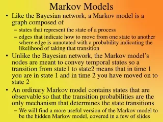
Markov Models • Like the Bayesian network, a Markov model is a graph composed of • states that represent the state of a process • edges that indicate how to move from one state to another where edge is annotated with a probability indicating the likelihood of taking that transition • Unlike the Bayesian network, the Markov model’s nodes are meant to convey temporal states so a transition from state1 to state2 means that in time 1 you are in state 1 and in time 2 you have moved on to state 2 • An ordinary Markov model contains states that are observable so that the transition probabilities are the only mechanism that determines the state transitions • We will find a more useful version of the Markov model to be the hidden Markov model, covered in a few of slides
A Markov Model • In the Markov model, we move from state to state based on simple probabilities • going from S3 to S2 has a likelihood of a32 • going from S3 to S3 has a likelihood of a33 • going from S3 to S4 has a likelihood of a34 • likelihoods are usually computed stochastically (statistically) We will use our Markov model to compute the likelihoods of a number of state transitions that might be of interest For instance, if we start in S1, what is the probability of going from S1 to S2 to S3 to S4 to S5 and back to S1? What is the probability of going from S1 to S1 to S1 to S1 to S2? Etc.
Example: Weather Forecasting • On any day, it will either be • rainy/snowy, cloudy or sunny • we have the following probability matrix to denote given any particular day, what the weather will be like tomorrow • so the probability, given today is sunny that tomorrow will be sunny is 0.8 • the probability, given today is rainy/snowy that tomorrow is cloudy is 0.2 • to compute a sequence, we multiply them together, so if today is sunny then the probability that the next two days will be sunny is 0.8 * 0.8, and the probability that the next three days will be cloudy is 0.1 * 0.1 * 0.1
Continued • Let’s assume today is cloudy and find the most likely sequence of three days • There are 8 such sequences • cloudy, cloudy, cloudy = .6 * .6 = .36 • cloudy, cloudy, rainy = .6 * .2 = .12 • cloudy, cloudy, sunny = .6 * .2 = .12 • cloudy, rainy, cloudy = .2 * .3 = .06 • cloudy, rainy, rainy = .2 * .4 = .08 • cloudy, rainy, sunny = .2 * .3 = .06 • cloudy, sunny, cloudy = .2 * .1 = .02 • cloudy, sunny, rainy = .2 * .1 = .02 • cloudy, sunny, sunny = .2 * .8 = .16 • for simplicity, assume rainy really means rainy or snowy • So the most likely sequence is three cloudy days in a row because today is cloudy • But what if we didn’t know what today would be?
Enhanced Example • Lets assume that the probability of the first day being cloudy = .5, rainy = .2 and sunny = .3 • These are our prior probabilities • Since we do not know the first day is cloudy, we now have 27 possible combinations • CCC, CCR, CCS, CRC, CRR, CRS, CSC, CSR, CSS, RCC, RCR, RCS, RRC, RRR, RRS, RSC, RSR, RSS, SCC, SCR, SCS, SRC, SRR, SRS, SSC, SSR, SSS • The most likely sequence now is SSS = .3 * .8 * .8 = .192 even though cloudy is the most likely first day (the probably for CCC = .5 * .6 * .6 = .18) • So, as with a Bayesian network, we have prior probabilities and multiply them by our conditional probabilities, which here are known as transitional probabilities
HMM • Most interesting AI problems cannot be solved by a Markov model because there are unknown states in our real world problems • in speech recognition, we can build a Markov model to predict the next word in an utterance by using the probabilities of how often any given word follows another • how often does “lamb” follow “little”? • A hidden Markov model (HMM) is a Markov model where the probabilities are actually probabilistic functions that are based in part on the current state, which is hidden (unknown or unobservable) • determining which transition to take will require additional knowledge than merely the state transition probabilities
Example: Speech Recognition • We have observations, the acoustic signal • But hidden from us is intention that created the signal • For instance, at time t1, we know what the signal looks like in terms of data, but we don’t know what the intended sound was (the phoneme or letter or word) • The goal in speech recognition is to identify the actual utterance (in terms of phonetic units or words) • but the phonemes/words are hidden to us • We add to our model hidden (unobservable) states and appropriate probabilities for transitions • the observables are not states in our network, but transition links • the hidden states are the elements of the utterance (e.g., phonemes), which is what we are trying to identify • we must search the HMM to determine what hidden state sequence best represents the input utterance
Example HMM • Here, X1, X2 and X3 are the hidden states • y1, y2, y3, y4 are observations • Aij are the transition probabilities of moving from state i to state j • bij make up the output probabilities from hidden node i to observation j – that is, what is the probability of seeing output yj given that we are in state xi? • Three problems associated with HMMs • Given HMM, compute the probability of a given output sequence • Given HMM and output sequence, compute most likely state transitions • 3. Given HMM and output sequence, compute the transition probabilities
Formal Definition of an HMM • The HMM is a graph, G = {V, E} • V is the set of vertices (nodes, states) • E is the set of directed edges, or the transitions between pairs of nodes • The HMM must have three sets of probabilities • Each node in V that can be the first state of a sequence has a prior probability (we can denote nodes that cannot be the first state as having prior probability = 0) • For each state transition (edge in E), we need a transition probability • For each node that has an associated observation, we need an output probability • Commonly an HMM will represent some k distinct time periods where the states at time i are completely connected to the states at time i-1 and time i+1 although not always • So, if there are n states and o possible observations at any time, there would be n prior probabilities, n*(k-1) transition probabilities, and n*o output probabilities
HMM Problem 1 • As stated previously, there are three problems that we can solve with our HMM • Problem 1: given an HMM and an output sequence, compute the probability of generating that particular output sequence (e.g., what is the likelihood of seeing this particular sequence of observations?) • We have an observation sequence O: O1 O2 O3 … Ok and states • Recall that we have 3 types of probabilities, prior probabilities, transition probabilities and output probabilities • We generate every possible sequence of hidden states through the HMM from 1 to k and compute • ps1 * bs1(O1) * as1s2 * bs2(O2) * as2s3 * bs3(O3) * … * ask-1sk * bsk(Ok) • Where p is the prior probability, a is the transition probability and b is the output probability • Since there are a number of sequences through the HMM, we compute the above probability for each sequence and sum them up
Brief Example We have 3 time units, t1, t2, t3 and each has 2 states, s1, s2 p(s1 at t1) = .8, p(s2 at t1) = .2 and there are 3 possible outputs , A, B, C Our transition probabilities a are p(s1, s1) = .7, p(s1, s2) = .3 and p(s2, s2) = .6, p(s2, s1) = .4 Our output probabilities are p(A, s1) = .5, p(B, s1) = .4, p(C, s1) = .1 p(A, s2) = .7, p(B, s2) = .3, p(B, s2) = 0 What is the probability of generating A, B, C? Possible sequences are s1 – s1 – s1: .8 * .5 * .7 * .4 * .3 * .1 = 0.00336 s1 – s1 – s2: .8 * .5 * .7 * .4 * .3 * 0 = 0.0 s1 – s2 – s1: .8 * .5 * .3 * .3 * .4 * .1 = 0.00144 s1 – s2 – s2: .8 * .5 * .3 * .3 * .6 * 0 = 0.0 s2 – s1 – s1: .2 * .7 * .4 * .4 * .7 * .1 = 0.001568 s2 – s1 – s2: .2 * .7 * .4 * .4 * .3 * 0 = 0.0 s2 – s2 – s1: .2 * .7 * .6 * .3 * .4 * .1 = 0.001008 s2 – s2 – s2: .2 * .7 * .6 * .3 * .6 * 0 = 0.0 Likelihood of the sequence A, B, C is 0.00336 + 0.00144 + 0.001568 + 0.001008 = 0.007376
More Efficient Solution • You might notice that there is a lot of repetition in our computation from the last slide • In fact, the number of sequences is O(k * nk) • When we compute s2 – s2 – s2, we had already computed s1 – s2 – s2, so the last half of the computation was already done • By using dynamic programming, we can reduce the number of computations • this is particularly relevant when the sequence is far longer than 3 states and has far more states per time unit than 2 • We use a dynamic programming algorithm called the Forward algorithm (see the next slide) • Even though we have a reasonably efficient means of solving problem 1, there is little need to solve this problem!
The Forward Algorithm • We solve the problem in three steps • The initialization step sets the probabilities of starting at each initial state at time 1 as • a1(i) = pi*bi(O1) for all states i • That is, the probability of starting at some state i is the prior probability for i * the output probability of seeing observation O1 from state i • The main step is recursive for all times after 1 • at+1(j) = [Sat(i)*aij]*bj(Ot+1) for all states j at time t+1 • That is, at time t+1, the probability of being at state j is the sum of all of the previous states at time t leading to state j (at(i)*aij) times the output probability of seeing Ot+1 at time t+1 • The final step is to sum up the probabilities of ending in each of the states at time n (sum up an(j) for all states j)
HMM Problem 2 • Given a sequence of observations, compute the optimal sequence of state transitions that would cause those observations • Alternatively, we could say that the optimal sequence best explains the observations • We need to define what we mean by “optimal” • The sequence that contains the most individual states with the highest likelihoods? • this sequence would contain the most states that appear to be correct states – notice that this solution does not take into account transitions • The sequence that contains the most number of correct pairs of states in the sequence • this would take into account transitions • or most number of correct triples, most number of correct quadruples, etc • The sequence that is the most likely (probable) overall
The Viterbi Algorithm • We do not know which of the sequences that were generated from problem 1 is actually the best path, we didn’t keep track of that • But through recursion and dynamic programming, we did keep track of portions of paths • So we will again use recursion • The recursive step works like this • Lets assume at some time t, we know the best paths to all states • At time t+1, we extend each of the best paths to time t by finding the best transition from time t to a state at t+1 • that is, we have to find a state at time t+1 such that the path to time t + transition to t+1 is best • we not only compute the new probability, but remember the path to this point
Viterbi Formally Described • Initialization step • d1(i) = pi*bi(O1) – same as in the forward algorithm • y1(i) = 0 – this array will represent the state that maximized our path leading to the prior state • The recursive step • dt+1(j) = max [dt(i)*aij]*bj(Ot+1) – here, we look at all of the previous states i at time t, and compute the state transition from t to t+1 that gives us the maximum value of dt(i)*aij–multiply that by the likelihood of this state being true given this time unit’s observation (see the next slide for a visual representation) • yt+1(j) = argmax [dt(i)*aij] –which i from the possible preceding states led to the maximum value? Store that
Continued • Termination step • p* = max[dn(i)] – the probability that the path selected is correct is the path that has the largest probability as found in the final time step from the last recursive call • q* = argmax [dn(i)] – this is the last state reached • Path backtracking • Now that we have found the best path, we backtrack using the array y starting at y[q*] until we reach time unit 1 At time t-1, we know the best paths to reach each of the states Now at time t, we look at each state si, and try to extend the path from t-1 to t
Example: Rainy and Sunny Days • Your colleague in another city either walks to work or drives every day and his decision is usually based on the weather • Given daily emails that include whether he has walked or driven to work, you want to guess the most likely sequence of whether the days were rainy or sunny • Two hidden states: rainy and sunny • Two observables: walking and driving • Assume equal likelihood of the first day being rainy or sunny • Transitional probabilities • rainy given yesterday was (rainy = .7, sunny = .3) • sunny given yesterday was (rainy = .4, sunny = .6) • Output (emission) probabilities • rainy given walking = .1, driving = .9 • sunny given walking = .8, driving = .2 • Given that your colleague walked, drove, walked, what is the most likely sequence of days?
Example Continued Day 1 is easy to compute, prior probability * output probability The initial path to get to day 1 is merely from state 0
Example Continued We determine that from day 1, it is more likely to reach sunny from rainy it is more likely to reach rainy from rainy as well, so day 2’s path to sunny is from rainy, and day 2’s path from rainy is from rainy
Example Concluded From day 2, it is more likely to reach sunny from sunny and it is more likely to reach rainy from sunny, but day 3’s most likely state is rainy. Since we reached the rainy state from sunny, and we reached Day 2’s sunny state from rainy, we now have the most likely path: rainy, sunny, rainy
Why Problem 2? • Unlike problem 1 which didn’t seem to have any useful AI applications, problem 2 is has many different types of AI problems that it could solve • This can be used to solve any number of credit assignment problems • given a speech signal, what was uttered (what phonemes or words were uttered)? • given a set of symptoms, what disease(s) is the patient suffering from? • given a misspelled word, which word was intended? • given a series of events, what caused them? • What we have are a set of observations (symptoms, manifestations) and we want to explain them • The HMM and Viterbi give us the ability to generate the best explanation where the term best means the most likely sequence through all of the states
How Do We Obtain our Probabilities? • We saw one of the issues involved Bayesian probabilities was gathering accurate probabilities • Like Bayesian probabilities, we need both prior probabilities and transition probabilities (the probability of moving from one state to another) • But here we also need output (or emission) probabilities • We can accumulate probabilities through counting • Given N cases, how many started at state s1? s2? s3? • although do we have enough cases to give us a good representative mix of probabilities? • Given N cases, out of all state transitions, how often do we move from s1 to s2? From s2 to s3? Etc • again, are there enough cases to give us a good distribution for transition probabilities? • How do we obtain the output probabilities? That is, how do we determine the likelihood of seeing output Oi in state Sj? • That’s trickier, and that’s where HMM problem 3 comes in
HMM Problem 3 • The final problem for HMMs is the most interesting and also the most challenging • Given HMM and output sequence, update the various probabilities • It turns out that there is an algorithm for modifying probabilities given a set of correct test cases • The algorithm is called the Baum-Welch algorithm (also known as the Estimation-Modification or EM algorithm) which uses as a component, the forward-backward algorithm • we already saw the forward portion of the forward algorithm, now we will take a look at the backward portion, which as you might expect, is very similar
Forward-Backward • We compute the forward probabilities as before • computing at(i) for each time unit t and each state i • The backward portion is similar but reversed • computing bt(i) for each time unit t and each state i • Initialization step • bt(i) = 1 – unlike the forward algorithm which used the prior probabilities, here we start at 1 (notice that we also start at time t, not time 1) • Recursive step • bt(i) = Saij * bj(Ot+1)*bt+1(j) – the probability of reaching state i at time t backwards, is the sum of transitions from all states at time t+1 * the probability of reaching state j at time t+1 * the probability of being at state j given output Ot+1 • this recursive step is almost the same as the step in the forward algorithm except that we use b instead of a
Baum-Welch (EM) • Now that we have computed all the forward and backward path probabilities, how do we use them? • First, we need to add a new value, the probability of being in state i at time t and transitioning to state j, which we will call xt(i, j) • Fortunately, once we have run the forward-backward algorithm, this is easy to compute as • xt(i, j) = at(i)*aij*bj(Ot+1)*bt+1(j) / denominator • Before describing the denominator, lets understand the numerator • this is the product of the probability of being at state i at time t multiplied by the transition probability of going from i to j multiplied by the output probability of seeing Ot+1 at time t+1 multiplied by the probability of being at state j at time t+1 • that is, it is the value derived by the forward algorithm for state i at time t * the value derived by the backward algorithm for state j at time t+1 * transition * output probabilities
Continued • The denominator is a normalizing value so that all of our probabilities xt(i, j) for all states i and j add up to 1 for time t • So this is merely the sum for all i and all j of at(i)*aij*bj(Ot+1)*bt+1(j) • Now we have some additional work • We add gt(i) = S xt(i, j) for all j at time t • This represents the expected number of times we are at state i at time t • If we sum up gt(i) for all times t, we have the number of expected times we are in state I • Now recall that we may have started with improper probabilities (prior, transition and output)
Re-estimation • By running the system on some test cases, we can accumulate probabilities of how likely a transition is, or how likely we start in a given state (prior probability) or how likely a state is for a given observation • At this point of the Baum Welch algorithm, we have accumulated a summation (from the previous slide) of various states we have visited • p(observation i | state j) = (expected number of times we saw observation i in the test case / number of times we achieved state j) (our observation probabilities) • p(state i | state j) = (expected number of transitions from i to j / number of times we were in state j) (our transition probabilities) • p(state i) = a1(i)*b1(i) / S[a1(i)*b1(i)] for all states i (this is the prior probability)
Continued • The math may be elusive, and the amount of computations required is intensive but now we have the ability to • Start with estimated probabilities (they don’t even have to be very good) • Use training examples to adjust the probabilities • And continue until the probabilities stabilize • that is, between iterations of Baum-Welch, they do not change (or their change is less than a given error rate) • So HMMs can be said to learn the proper probabilities through training examples • Each training example is merely the observations and the expected output (hidden states) • The better the initial probabilities, the more likely it will be that the algorithm will converge to a stable state quickly, the worse the initial probabilities, the longer it will take
Example: Determining the Weather • Here, we have an HMM that attempts to determine for each day, whether it was hot or cold • observations are the number of ice cream cones a person ate (1-3) • the following probabilities are estimates that we will correct through learning
Computing a Path Through the HMM • Assume we know that the person ate in order, the following cones: 2, 3, 3, 2, 3, 2, 3, 2, 2, 3, 1, … • What days were hot and what days were cold? • P(day i is hot | j cones) = ai(H) * bi(H) / (ai(C) * bi(C) + ai(H) * bi(H) ) • a(H), b(H), a(C) and b(C) were all computed using the forward-backward algorithm • We started with guesses for our initial probabilities • Now that we have run one iteration of forward-backward, we can apply re-estimation • Sum up the values of our computations P(C | 1)s and P(C) • Recompute P(1 | C) = sum P(C | 1) / P(C) • we also do the same for P(C | 2), and P(C | 3) to compute P(2 | C) and P(3 | C) as well as the hot days for P(1 | H), P(2 | H), P(3 | H) • And we recompute P(C | C), P(C | H), etc • Now our probabilities are more accurate (although not necessarily correct)
Continued • We update the probabilities (see below) • since our original probabilities will impact how good these estimates are, we repeat the entire process with another iteration of forward-backward followed by re-estimation • we continue to do this until our probabilities converge into a stable state • So, our initial probabilities will be important only in that they will impact the number of iterations required to reach these stable probabilities
Convergence and Perplexity • This system converged in 10 iterations to the probabilities shown in the table below • Our original transition probabilities were part of our “model” of weather • updating them is fine, but what would happen if we had started with different probabilities? say p(H|C) = .25 instead of .1? • the perplexity of a model is essentially the degree to which we will be surprised by the results of our model because of the “guesses” we made when assigning a random probability like p(H|C) • We want our model to have a minimal perplexity so that it is most realistic
Two Problems With HMMs • There are two primary problems with using HMMs • The first is minor – what if a probability (whether output or transition) is 0? • Because we are multiplying probabilities together, this would cause a path that goes through the state will have a probability of 0 and so will never be selected • To get around this problem, we will replace any 0 probabilities with some minimum probability (say .001) • The other is the complexity of the search • Imagine we are using an HMM for speech recognition where the hidden states are the possible phonemes (say there are 30 of them) and the utterance consists of some 100 phonemes (perhaps 20 words) • Recall that the complexity for the forward algorithm is O(T*NT) where N is 30 and T is 100! Ouch • So we might use a beam search to reduce the number of possible paths searched
Beam Search • A beam search is a combination of the heuristic search idea along with a breadth-first search • The beam search algorithm examines all of the next states accessible and evaluates them • for an HMM, the evaluation is the probability a or b depending on whether we are doing a forward or backward pass • In order to reduce the complexity of the search, only some of the states at this time interval are retained • we might either keep the top k where k is a constant (known as the beam width) or we can use a threshold value and prune away states that do not exceed the threshold value • if we discard a state, we are actually discarding the entire path that led us to that state (recall that the path would be the path that had the highest probability leading to that particular state at that time)
Forms of HMMs • One of the most common form of HMM is called an Ergodic model – this is a fully connected model, that is, every state has an edge to every other state • From ealier in the lecture, we saw a slide of examples – the bull/bear market and the cloudy/sunny/rainy day are examples • The weather/ice cream cone example could be thought of as an Ergodic model, but instead we would prefer to envision each day as being in a new state, so this leads us to the Forward Trellis model Each variant of HMM has its own training algorithms although they are all based on Baum-Welch
Bakis and Factorial HMMs • The Bakis model is one used to denote precise temporal changes where states transition left to right across the model where each state represents a new time unit • States may also loop back onto themselves • This is often used in speech recognition for instance to represent portions of a phonetic unit • see below to the left • Factorial HMMs – when the system is so complex that a given state cannot represent the process of a single state in the model • at time i, there will be multiple states, all of which lead to multiple successor states and all of which have emission probabilities from the observations input (see the figure below)
Hierarchical HMM • We use this model when each state is itself a self-contained probabilistic model including their own hidden nodes • That is, a state has its own internal HMM • The rationale for having a HHMM is that each state can represent a sequence of observations instead of a one-to-one mapping of observation and state • For instance, q2 might consist of 3 or more observations as shown in the figure
N-Grams • N-Gram HMMs – the transition probabilities here are not just from the previous time unit, but from n-1 prior time units • The N-gram is primarily used in natural language understanding or genetics types of problems where we can accumulate the transition probabilities from some corpus of data • The bi-gram is the most common form of n-gram used in natural language understanding • To the right is some bigram data for the frequency of two-letter pairs in English (out of 2000 words) • Tri-grams are also somewhat commonly used but it is rare to go beyond tri-grams TH 50 AT 25 ST 20 ER 40 EN 25 IO 18 ON 39 ES 25 LE 18 AN 38 OF 25 IS 17 RE 36 OR 25 OU 17 HE 33 NT 24 AR 16 IN 31 EA 22 AS 16 ED 30 TI 22 DE 16 ND 30 TO 22 RT 16 HA 26 IT 20 VE 16
Applications for HMMs • The first impressive use of HMMs in AI was for speech recognition (in the late 80s) • Since then, a lot of other applications have been tested • Hand written character recognition • Natural language understanding • word sense disambiguation • machine translation • word matching (for misspelled words) • semantic tagging of words (could be useful for the semantic web) • Bioinformatics (e.g., protein structure predictions, gene analysis and sequencing predictions) • Market predictions • Diagnosis of mechanical systems