Modeling and Solving LP Problems in a Spreadsheet
Chapter 3. Modeling and Solving LP Problems in a Spreadsheet. Introduction. Solving LP problems graphically is only possible when there are two decision variables Few real-world LP have only two decision variables Fortunately, we can now use spreadsheets to solve LP problems.

Modeling and Solving LP Problems in a Spreadsheet
E N D
Presentation Transcript
Chapter 3 Modeling and Solving LP Problems in a Spreadsheet
Introduction • Solving LP problems graphically is only possible when there are two decision variables • Few real-world LP have only two decision variables • Fortunately, we can now use spreadsheets to solve LP problems
Spreadsheet Solvers • The company that makes the Solver in Excel, Lotus 1-2-3, and Quattro Pro is Frontline Systems, Inc. Check out their web site: http://www.solver.com • Other packages for solving MP problems: AMPL LINDO CPLEX MPSX
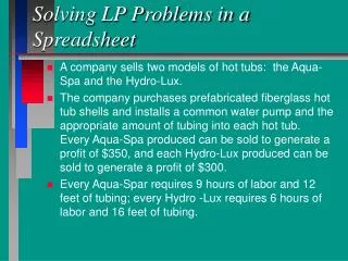
Let’s Implement a Model for the Blue Ridge Hot Tubs Example... MAX: 350X1 + 300X2 } profit S.T.: 1X1 + 1X2 <= 200 } pumps 9X1 + 6X2 <= 1566 } labor 12X1 + 16X2 <= 2880 } tubing X1, X2 >= 0 } nonnegativity See file Fig3-1.xls for implementing the model
How Solver Views the Model • Target cell - the cell in the spreadsheet that represents the objective function • Changing cells - the cells in the spreadsheet representing the decision variables • Constraint cells - the cells in the spreadsheet representing the LHS formulas on the constraints
Model 1 Model 2 Model 3 Number ordered 3,000 2,000 900 Hours of wiring/unit 2 1.5 3 Hours of harnessing/unit 1 2 1 Cost to Make $50 $83 $130 Cost to Buy $61 $97 $145 Make vs. Buy Decisions:The Electro-Poly Corporation • Electro-Poly is a leading maker of slip-rings. • A $750,000 order has just been received. • The company has 10,000 hours of wiring capacity and 5,000 hours of harnessing capacity.
Defining the Decision Variables M1 = Number of model 1 slip rings to make in-house M2 = Number of model 2 slip rings to make in-house M3 = Number of model 3 slip rings to make in-house B1 = Number of model 1 slip rings to buy from competitor B2 = Number of model 2 slip rings to buy from competitor B3 = Number of model 3 slip rings to buy from competitor
Defining the Objective Function Minimize the total cost of filling the order. MIN: 50M1+ 83M2+ 130M3+ 61B1+ 97B2+ 145B3
Defining the Constraints • Demand Constraints M1 + B1 = 3,000 } model 1 M2 + B2 = 2,000 } model 2 M3 + B3 = 900 } model 3 • Resource Constraints 2M1 + 1.5M2 + 3M3 <= 10,000 } wiring 1M1 + 2.0M2 + 1M3 <= 5,000 } harnessing • Nonnegativity Conditions M1, M2, M3, B1, B2, B3 >= 0 • See file Fig3-17.xls for implementing the model
Years to Company Return Maturity Rating Acme Chemical 8.65% 11 1-Excellent DynaStar 9.50% 10 3-Good Eagle Vision 10.00% 6 4-Fair Micro Modeling 8.75% 10 1-Excellent OptiPro 9.25% 7 3-Good Sabre Systems 9.00% 13 2-Very Good An Investment Problem:Retirement Planning Services, Inc. • A client wishes to invest $750,000 in the following bonds.
Investment Restrictions • No more than 25% can be invested in any single company. • At least 50% should be invested in long-term bonds (maturing in 10+ years). • No more than 35% can be invested in DynaStar, Eagle Vision, and OptiPro.
Defining the Decision Variables X1 = amount of money to invest in Acme Chemical X2 = amount of money to invest in DynaStar X3 = amount of money to invest in Eagle Vision X4 = amount of money to invest in MicroModeling X5 = amount of money to invest in OptiPro X6 = amount of money to invest in Sabre Systems
Defining the Objective Function Maximize the total annual investment return: MAX: .0865X1+ .095X2+ .10X3+ .0875X4+ .0925X5+ .09X6
Defining the Constraints • Total amount is invested X1 + X2 + X3 + X4 + X5 + X6 = 750,000 • No more than 25% in any one investment Xi <= 187,500, for all i • 50% long term investment restriction. X1 + X2 + X4 + X6 >= 375,000 • 35% Restriction on DynaStar, Eagle Vision, and OptiPro. X2 + X3 + X5 <= 262,500 • Nonnegativity conditions Xi >= 0 for all i • See file Fig3-20.xls for implementing the model
Processing Plants Groves Distances (in miles) Supply Capacity 21 Mt. Dora Ocala 200,000 275,000 1 4 50 40 35 30 Eustis Orlando 600,000 400,000 2 5 22 55 20 Clermont Leesburg 225,000 300,000 3 6 25 A Transportation Problem: Tropicsun
Defining the Decision Variables Xij= # of bushels shipped from node ito node j Specifically, the nine decision variables are: X14 = # of bushels shipped from Mt. Dora (node 1) to Ocala (node 4) X15 = # of bushels shipped from Mt. Dora (node 1) to Orlando (node 5) X16 = # of bushels shipped from Mt. Dora (node 1) to Leesburg (node 6) X24 = # of bushels shipped from Eustis (node 2) to Ocala (node 4) X25 = # of bushels shipped from Eustis (node 2) to Orlando (node 5) X26 = # of bushels shipped from Eustis (node 2) to Leesburg (node 6) X34 = # of bushels shipped from Clermont (node 3) to Ocala (node 4) X35 = # of bushels shipped from Clermont (node 3) to Orlando (node 5) X36 = # of bushels shipped from Clermont (node 3) to Leesburg (node 6)
Defining the Objective Function Minimize the total number of bushel-miles. MIN: 21X14 + 50X15 + 40X16 + 35X24 + 30X25 + 22X26 + 55X34 + 20X35 + 25X36
Defining the Constraints • Capacity constraints X14 + X24 + X34 <= 200,000 } Ocala X15 + X25 + X35 <= 600,000 } Orlando X16 + X26 + X36 <= 225,000 } Leesburg • Supply constraints X14 + X15 + X16 = 275,000 } Mt. Dora X24 + X25 + X26 = 400,000 } Eustis X34 + X35 + X36 = 300,000 } Clermont • Nonnegativity conditions Xij>= 0 for all iandj • See file Fig3-24.xls for implementing the model
Percent of Nutrient in Nutrient Feed 1 Feed 2 Feed 3 Feed 4 Corn 30% 5% 20% 10% Grain 10% 3% 15% 10% Minerals 20% 20% 20% 30% Cost per pound $0.25 $0.30 $0.32 $0.15 A Blending Problem:The Agri-Pro Company • Agri-Pro has received an order for 8,000 pounds of chicken feed to be mixed from the following feeds. • The order must contain at least 20% corn, 15% grain, and 15% minerals.
Defining the Decision Variables X1 = pounds of feed 1 to use in the mix X2 = pounds of feed 2 to use in the mix X3 = pounds of feed 3 to use in the mix X4 = pounds of feed 4 to use in the mix
Defining the Objective Function Minimize the total cost of filling the order. MIN: 0.25X1 + 0.30X2 + 0.32X3 + 0.15X4
Defining the Constraints • Produce 8,000 pounds of feed X1 + X2 + X3 + X4 = 8,000 • Mix consists of at least 20% corn (0.3X1 + 0.5X2 + 0.2X3 + 0.1X4)/8000 >= 0.2 • Mix consists of at least 15% grain (0.1X1 + 0.3X2 + 0.15X3 + 0.1X4)/8000 >= 0.15 • Mix consists of at least 15% minerals (0.2X1 + 0.2X2 + 0.2X3 + 0.3X4)/8000 >= 0.15 • Nonnegativity conditions X1, X2, X3, X4 >= 0
A Comment About Scaling • Notice the coefficient for X2 in the ‘corn’ constraint is 0.05/8000 = 0.00000625 • As Solver runs, intermediate calculations are made that make coefficients larger or smaller. • Storage problems may force the computer to use approximations of the actual numbers. • Such ‘scaling’ problems sometimes prevents Solver from being able to solve the problem accurately. • Most problems can be formulated in a way to minimize scaling errors...
Re-Defining the Decision Variables X1 = thousands of pounds of feed 1 to use in the mix X2 = thousands of pounds of feed 2 to use in the mix X3 = thousands of pounds of feed 3 to use in the mix X4 = thousands of pounds of feed 4 to use in the mix
Re-Defining the Objective Function Minimize the total cost of filling the order. MIN: 250X1 + 300X2 + 320X3 + 150X4
Re-Defining the Constraints • Produce 8,000 pounds of feed X1 + X2 + X3 + X4 = 8 • Mix consists of at least 20% corn (0.3X1 + 0.5X2 + 0.2X3 + 0.1X4)/8 >= 0.2 • Mix consists of at least 15% grain (0.1X1 + 0.3X2 + 0.15X3 + 0.1X4)/8 >= 0.15 • Mix consists of at least 15% minerals (0.2X1 + 0.2X2 + 0.2X3 + 0.3X4)/8 >= 0.15 • Nonnegativity conditions X1, X2, X3, X4 >= 0
Scaling: Before and After • Before: • Largest constraint coefficient was 8,000 • Smallest constraint coefficient was 0.05/8 = 0.00000625. • After: • Largest constraint coefficient is 8 • Smallest constraint coefficient is 0.05/8 = 0.00625. • The problem is now more evenly scaled! • See file Fig3-28.xls for implementing the model
The “Assume Linear Model” Option • The Solver Options dialog box has an option labeled “Assume Linear Model”. • This option makes Solver perform some tests to verify that your model is in fact linear. • These test are not 100% accurate & may fail as a result of a poorly scaled model. • If Solver tells you a model isn’t linear when you know it is, try solving it again. If that doesn’t work, try re-scaling your model.