Download
1 / 39
390 likes | 438 Vues
Explore the mathematics and methods of clustering gene expression profiles using probabilistic agglomerative clustering. Learn about the scoring method, double clustering, and practical applications across various disciplines including marketing and earthquake studies. Understand the difference between partitioning and hierarchical clustering methods and how to choose the right approach for your dataset. Discover the merits of a good clustering solution and the Gaussian distribution function.

E N D
PCluster: Probabilistic Agglomerative Clustering of Gene Expression Profiles Nir Friedman Presenting: Inbar Matarasso 09/05/2005 The School of Computer Science Tel – Aviv University
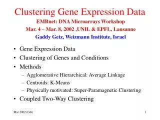
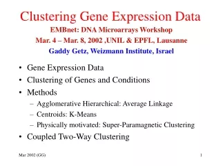
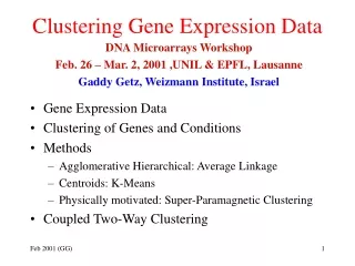
Outline • A little about clustering • Mathematics background • Introduction • The problem • Notation • Scoring Method • Agglomerative clustering • Double clustering • Conclusion
A little about clustering • Partition entities (genes) into groups called clusters (according to similarity in their expression profiles across the probed conditions). • Cluster are homogeneous and well-separated. • Clustering problem arise in numerous disciplines including biology, medicine, psychology, economics.
Clustering – why? • Reduce the dimensionality of the problem – identify the major patterns in the dataset • Pattern Recognition • Image Processing • Economic Science (especially market research) • WWW • Document classification • Cluster Weblog data to discover groups of similar access patterns
Examples of Clustering Applications • Marketing: Help marketers discover distinct groups in their customer bases, and then use this knowledge to develop targeted marketing programs • Insurance: Identifying groups of motor insurance policy holders with a high average claim cost • Earth-quake studies: Observed earth quake epicenters should be clustered along continent faults
Types of clustering methods • How to choose a particular method? • The type of output desired • The known performance of method with particular types of data • The hardware and software facilities available • The size of the dataset. • In general , clustering methods may be divided into two categories based on the cluster structure which they produce: Partitioning Methods, Hierarchical Agglomerative methods
Partitioning Methods • Partition the objects into a prespecified number of groups K • Iteratively reallocate objects to clusters until some criterion is met (e.g. minimize within cluster sums of squares) • Examples: k-means, partitioning around medoids (PAM), self-organizing maps (SOM), model-based clustering
Partitioning Methods • Result: M clusters, each object belonging to one cluster • Single Pass: • Make the first object the centroid for the first cluster. • For the next object, calculate the similarity, S, with each existing cluster centroid, using some similarity coefficient. • If the highest calculated S is greater than some specified threshold value, add the object to the corresponding cluster and re determine the centroid; otherwise, use the object to initiate a new cluster. If any objects remain to be clustered, return to step 2.
Partitioning Methods • This method requires only one pass through the dataset • The time requirements are typically of order O(NlogN) for order O(logN) clusters. • A disadvantage is that the resulting clusters are not independent of the order in which the documents are processed, with the first clusters formed usually being larger than those created later in the clustering run
Hierarchical Clustering • Produce a dendrogram • Avoid prespecification of the number of clusters K • The tree can be built in two distinct ways: • Bottom-up: agglomerative clustering • Top-down: divisive clustering
{1,2,3,4,5} {1,2,3} {4,5} {1,2} g1 g2 g3 g4 g5 Hierarchical Clustering • Organize the genes in a structure of a hierarchical tree • Initial step: each gene is regarded as a cluster with one item • Find the 2 most similar clusters and merge them into a common node • The length of the branch is proportional to the distance • Iterate on merging nodes until all genes are contained in one cluster- the root of the tree.
Partitioning vs. Hierarchical • Partitioning • Advantage: Provides clusters that satisfy some optimality criterion (approximately) • Disadvantages: Need initial K, long computation time • Hierarchical • Advantage: Fast computation (agglomerative) • Disadvantages: Rigid, cannot correct later for erroneous decisions made earlier
Mathematical evaluation of clustering solution Merits of a ‘good’ clustering solution: • Homogeneity: • Genes inside a cluster are highly similar to each other. • Average similarity between a gene and the center (average profile) of its cluster. • Separation: • Genes from different clusters have low similarity to each other. • Weighted average similarity between centers of clusters. • These are conflicting features: increasing the number of clusters tends to improve with-in cluster Homogeneity on the expense of between-cluster Separation
Gaussian Distribution Function • Large number of events • describes physical events • approximates the exact binomial distribution of events
Bayes' Theorem • p(A|X) = p(X|A)*p(A) p(X|A)*p(A) + p(X|~A)*p(~A) • 1% of women at age forty who participate in routine screening have breast cancer. 80% of women with breast cancer will get positive mammographies. 9.6% of women without breast cancer will also get positive mammographies. A woman in this age group had a positive mammography in a routine screening. What is the probability that she actually has breast cancer?
Bayes' Theorem • The correct answer is 7.8%, obtained as follows: Out of 10,000 women, 100 have breast cancer; 80 of those 100 have positive mammographies. From the same 10,000 women, 9,900 will not have breast cancer and of those 9,900 women, 950 will also get positive mammographies. This makes the total number of women with positive mammographies 950+80 or 1,030. Of those 1,030 women with positive mammographies, 80 will have cancer. Expressed as a proportion, this is 80/1,030 or 0.07767 or 7.8%.
Bayes' Theorem • to find the chance that a woman with positive mammography has breast cancer, we computed: p(positive|cancer)*p(cancer) p(positive|cancer)*p(cancer) + p(positive|~cancer)*p(~cancer) • which isp(positive&cancer) / [p(positive&cancer) + p(positive&~cancer)] • which isp(positive&cancer) / p(positive) • which isp(cancer|positive)
Bayes' Theorem • The original proportion of patients with breast cancer is known as the prior probability. The chance that a patient with breast cancer gets a positive mammography, and the chance that a patient without breast cancer gets a positive mammography, are known as the two conditional probabilities. Collectively, this initial information is known as the priors. The final answer - the estimated probability that a patient has breast cancer, given that we know she has a positive result on her mammography - is known as the revised probability or the posterior probability.
Bayes' Theorem p(A|X) = p(A|X) p(A|X) = p(X&A) p(X) p(A|X) = p(X&A) p(X&A) + p(X&~A) p(A|X) = p(X|A)*p(A) p(X|A)*p(A) + p(X|~A)*p(~A)
Introduction • A central problem in analysis of gene expression data is clustering of genes with similar expression profiles. • We are going to get familiar with an hierarchical clustering procedure that is based on simple probabilistic model. • Genes that are expressed similarly in each group of conditions are clustered together.
The problem • The goal of clustering is identify groups of genes with “similar” expression patterns. • A group of genes are clustered together if their measured expression values could have been sampled from the same stochastic source with a high probability. • The user specifies in advance a partition of the experimental conditions
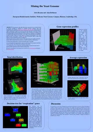
Clustering Gene Expression Data • Cluster genes , e.g. to (attempt to) identify groups of co-regulated genes • Cluster samples, e.g. to identify tumors based on profiles • Cluster both at the same time • Can be helpful for identifying patterns in time or space • Useful (essential?) when seeking new subclasses of samples • Can be used for exploratory purposes
Notation • a matrix of gene expression measurement: D = {eg,c : gєGenes, cєConds} • Genes is a set genes, and Conds is a set of conditions
Scoring Method • partition C = {C1, … ,Cm} of conditions in Conds and a partition G = {G1 , … , Gn} of genes in Genes. • We want to score the combined partition. • Assumption:g and g’ are in the same gene cluster, and c and c’ in the same condition cluster, then the expression value eg,c and eg’,c’ are sampled from the same distribution.
Scoring Method • Likelihood function: • Where θi,k are the parameters that describe the expression of genes in Gi in conditions in Ck. • L(G,C,θ:D) = L(G,C,θ:D’) for any choice of G and θ.
Scoring Method • Parameterization for expression is using a Gaussian distribution.
Scoring Method • Using the previous Parameterization for each data we choose the best parameter sets. • To compensate for this overestimate we use the Bayesianapproach, and average the likelihood over all of them.
Scoring Method - Summary • Local score of a particular cell:
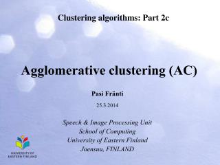
Agglomerative Clustering • Given a partition C = {C1, … ,Cm} of conditions. • One approach to learn a clustering of genes is using an agglomerative procedure.
Agglomerative Clustering • G(1) ={G1, … ,G|Genes|} where each Gi is a singleton. • While t < |Genes| and G(t) contains a single cluster. • Compute the change in the score that results from merging the clusters Gi and Gj
Agglomerative Clustering • Choose (it,jt) to be the pair of clusters whose merger is the most beneficial according to the score: • Define: • O(|Genes|2|C|)
Double Clustering • We want the procedure to select for us the best partition: • Track the sequence of partitions G(1),…, G|Genes|. • Select the partition with the highest score. • In theory: the maximum likelihood score should select G(1) • In Practice: it selects a partition in a much later stage. • Intuition: the best scoring partition strikes a tradeoff between finding groups of genes, so that each is homogeneous, and there distinct differences between them.
Double Clustering • Cluster both genes and conditions at the same time: • start with some partition of the conditions (say the one where each is a singleton). • perform gene agglomeration • select the “best” scoring gene partition • fix this gene partition • perform agglomeration on conditions • Intuitively, each step improves the score, and thus this procedure should converge.
particular features of our algorithm • We can measure a large amount of genes. • The agglomerative clustering algorithm returns a hierarchical partition that describes similarities at different scales. • We use a likelihood function rather than a measure of similarity. • The user specifies in advance a partition of experimental conditions.
Conclusion • Partition entities into groups called clusters . • Cluster are homogeneous and well-separated. • Bayes' Theorem p(A|X) = p(X|A)*p(A) p(X|A)*p(A) + p(X|~A)*p(~A) • Partitions: C = {C1, … ,Cm}, G = {G1 , … , Gn} we want to score the combined partition. • Likelihood function:
Conclusion • Agglomerative Clustering • The main advantage of this procedure is that it can take as input the “relevant” distinctions among the conditions
References [1] N. Friedman. PCluster: Probabilistic Agglomerative Clustering of Gene Expression Profiles. 2003 [2] A. Ben-Dor, R. Shamir, and Z. Yakhini. Clustering gene expression patterns. J. Comp. Bio., 6(3-4):281–97, 1999. [3] M. B. Eisen, P. T. Spellman, P. O. Brown, and D. Botstein. Cluster analysis and display of genomewide expression patterns. PNAS, 95(25):14863–8, 1998. [4] Eliezer Yudkowsky. An Intuitive Explanation of Bayesian Reasoning. 2003