Clustering Algorithms for Categorical Data Sets
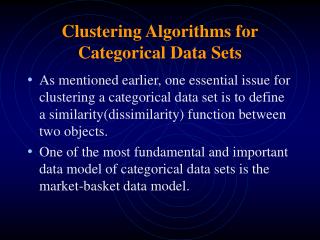
Clustering Algorithms for Categorical Data Sets. As mentioned earlier, one essential issue for clustering a categorical data set is to define a similarity(dissimilarity) function between two objects.

Clustering Algorithms for Categorical Data Sets
E N D
Presentation Transcript
Clustering Algorithms for Categorical Data Sets • As mentioned earlier, one essential issue for clustering a categorical data set is to define a similarity(dissimilarity) function between two objects. • One of the most fundamental and important data model of categorical data sets is the market-basket data model.
The Market-Basket Data Model • In the data model, there is a set of objects {O1, O2,…, On} and a set of transactions {T1, T2,…, Tm}. Each transaction is actually is subset of the object set. • A market-basket data set is typically represented by a 2-dimensional table, in which each entry is either 0 or 1.
Data Sets with the Market-Basket Data Model • A record of purchasing transactions. • A record of web site accesses. • A record of course enrollment.
Clustering Objects in a Market-Basket Data Set • In this problem, it is assumed that each transaction is an independent event. • The commonly used measures of similarity include: • Jacard coefficient. • Mutual information.
Once the similarity between each pair of objects has been determined, then we may apply algorithms such as single-link and complete-link to cluster the objects. • Experiment results shows that the complete-link algorithm generally yield better clustering quality than the single-link algorithm.
An Example • Given the following web access record, we may cluster the web sites accordingly.
Based on the Jacard coefficient, we have the following similarity measurements: sim(s1, s2) = 1/5 sim(s1, s3) = 3/4 sim(s1, s4) = 2/5 sim(s1, s5) = 3/5 sim(s2, s3) = 0 sim(s2, s4) = 2/3 sim(s2, s5) = 1/2 sim(s3, s4) = 1/5 sim(s3, s5) = 2/5 sim(s4, s5) = 3/5
If we employ the complete-link algorithm, then we have the following cluster result: ½ 2/3 ¾ s1 s3 s2 s4 s5
We may use the chi-square statistics as the similarity measure. However, we need to consider whether the accesses to two web sites are positively correlated or negatively correlated. • For example:
The Object-Attribute Data Model • In the data model, there is a set of objects {O1, O2,…, On} and a set of attributes {A1, A2,…, Am}. Each attribute has a number of possible values. • For example, we may characterize a person by education background, profession, marriage status, …etc.
Attributes Attributes … Ai=v2 Ai=vk Ai=v1 Ai Objects Objects v1 v2 : : vk • If each attribute has exactly two possible values, then the object-attribute data model is degenerated to the market-basket data model. • An object-attribute data set can be transformed to a market-basket data set as the following example shows.
The ROCK algorithm • A categorical data clustering algorithm that takes into account node connectivity. • In ROCK, each object is represented by a node. • Two nodes are connected by an edge if the similarity between the corresponding objects exceeds a threshold.
Let link(ni, nj) of two nodes ni and nj denote the number of common neighbors of these two nodes. • Given a data set and an integer number k, the ROCK algorithm partitions the objects into k clusters so that the following function is maximized.
The ROCK algorithm works bottom-up by merging the pair of clusters that has maximum goodness measurement
Fundamental of the Criteria Functions • Assume that the expected number of edges at a node in cluster Ci is |Ci|f(). • Then, the expected number of links contributed by a node in Ci is • Therefore, the expected number of links in Ci is
The Pseudo-code of the ROCK Algorithm • procedure cluster(S,k)beginlink := compute_links(S) for eachsSdoq[s] := build_local_heap(link,s)Q := build_global_head(S,q) whilesize(Q) > kdo {u := extract_max(Q)v := max(q[u]) delete(Q,v)w := merge(u,v) for eachxq[u]q[v] do {link[x,w] := link[x,u] + link[x,v] delete(q[x],u); delete(q[x],v) insert(q[x],w,g(w,x)); insert(q[w],x,g(w,x)) update(Q,x,q[x]) } insert(Q,w,q[x]) deallocate(q[u]); deallocate(q[v]) }end
The COBWEB Conceptual Clustering Algorithm • The COBWEB algorithm was developed by machine learning researchers in the 1980s for clustering objects in a object-attribute data set. • The COBWEB algorithm yields a clustering dendrogram called classification tree that characterizes each cluster with a probabilistic description.
The Category Utility Function • The COBWEB algorithm operates based on the so-called category utility function (CU) that measures clustering quality. • If we partition a set of objects into m clusters, then the CU of this particular partition is
Insights of the CU Function • For a given object in cluster Ck, if we guess its attribute values according to the probabilities of occurring, then the expected number of attribute values that we can correctly guess is
Given an object without knowing the cluster that the object is in, if we guess its attribute values according to the probabilities of occurring, then the expected number of attribute values that we can correctly guess is
P(Ck)is incorporated in the CU function to give paper weighting to each cluster. • Finally, m is placed in the denominator to prevent over-fitting.
Operation of the COBWEB algorithm • The COBWEB algorithm constructs a classification tree incrementally by inserting the objects into the classification tree one by one. • When inserting an object into the classification tree, the COBWEB algorithm traverses the tree top-down starting from the root node.
At each node, the COBWEB algorithm considers 4 possible operations and select the one that yields the highest CU function value: • insert. • create. • merge. • split.
Insertion means that the new object is inserted into one of the existing child nodes. The COBWEB algorithm evaluates the respective CU function value of inserting the new object into each of the existing child nodes and selects the one with the highest score. • The COBWEB algorithm also considers creating a new child node specifically for the new object.
P P Merge … … … … … A B N … A B • The COBWEB algorithm considers merging the two existing child nodes with the highest and second highest scores.
P P Split … … … … … A B N … A B • The COBWEB algorithm considers spliting the existing child node with the highest score.
The COBWEB Algorithm Cobweb(N, I) If N is a terminal node, Then Create-new-terminals(N, I) Incorporate(N,I). Else Incorporate(N, I). For each child C of node N, Compute the score for placing I in C. Let P be the node with the highest score W. Let Q be the node with the second highest score. Let X be the score for placing I in a new node R. Let Y be the score for merging P and Q into one node. Let Z be the score for splitting P into its children. If W is the best score, Then Cobweb(P, I) (place I in category P). Else if X is the best score, Then initialize R’s probabilities using I’s values (place I by itself in the new category R). Else if Y is the best score, Then let O be Merge(P, R, N). Cobweb(O, I). Else if Z is the best score Then Split(P, N). Cobweb(N, I). Input: The current node N in the concept hierarchy. An unclassified (attribute-value) instance I. Results: A concept hierarchy that classifies the instance. Top-level call: Cobweb(Top-node, I). Variables: C, P, Q, and R are nodes in the hierarchy. U, V, W, and X are clustering (partition) scores.
Auxiliary COBWEB Operations Variables: N, O, P, and R are nodes in the hierarchy. I is an unclassified instance. A is a nominal attribute. V is a value of an attribute. Incorporate(N, I) update the probability of category N. For each attribute A in instance I, For each value V of A, Update the probability of V given category N. Create-new-terminals(N, I) Create a new child M of node N. Initialize M’s probabilities to those for N. Create a new child O of node N. Initialize O’s probabilities using I’s value. Merge(P, R, N) Make O a new child of N. Set O’s probabilities to be P and R’s average. Remove P and R as children of node N. Add P and R as children of node O. Return O. Split(P, N) Remove the child P of node N. Promote the children of P to be children of N.
Probability-Based Clustering • The foundation of the probability-based clustering approach is based on a so-called finite mixture model. • A mixture is a set of k probability distributions, each of which governs the attribute values distribution of a cluster.
A 2-Cluster Example of the Finite Mixture Model • In this example, it is assumed that there are two clusters and the attribute value distributions in both clusters are normal distributions. N(1,12) N(2,22)
The Data Set • A 51 B 62 B 64 A 48 A 39 A 51 • A 43 A 47 A 51 B 64 B 62 A 48 • B 62 A 52 A 52 A 51 B 64 B 64 • B 64 B 64 B 62 B 63 A 52 A 42 • A 45 A 51 A 49 A 43 B 63 A 48 • A 42 B 65 A 48 B 65 B 64 A 41 • A 46 A 48 B 62 B 66 A 48 • A 45 A 49 A 43 B 65 B 64 • A 45 A 46 A 40 A 46 A 48
Operation of the EM Algorithm • The EM algorithm is to figure out the parameters for the finite mixture model. • Let {s1, s2,…, sn} denote the the set of samples. • In this example, we need to figure out the following 5 parameters: 1, 1, 2, 2, P(C1).
For a general 1-dimensional case that has k clusters, we need to figure out totally 2k+(k-1) parameters. • The EM algorithm begins with an initial guess of the parameter values.
Then, the probabilities that sample si belongs to these two clusters are computed as follow:
The new estimated values of parameters are computed as follows.
The process is repeated until the clustering results converge. • Generally, we attempt to maximize the following likelihood function:
Once we have figured out the approximate parameter values, then we assign sample si into C1, if • Otherwise, si is assigned into C2.
The Finite Mixture Model for Multiple Attributes • The finite mixture model described above can be easily generalized to handle multiple independent attributes. • For example, in a case that has two independent attributes, then the distribution function of cluster j is of form:
Assume that there are 3 clusters in a 2-dimensional data set. Then, we have 14 parameters to be determined: x1, y1, x1, y1, x2, y2, x2, y1, x3, y3, x3, y3, P(C1), and P(C2). • The probability that sample si belongs to Cj is:
The new estimated values of the parameters are computed as follows:
Limitation of the Finite Mixture Model and the EM Algorithm • The finite mixture model and the EM algorithm generally assume that the attributes are independent. • Approaches have been proposed for handling correlated attributes. However, these approaches are subject to further limitations.
Generalization of the Finite Mixture Model and the EM Algorithm • The finite mixture model and the EM algorithm can be generalized to handle other types of probability distributions. • For example, if we want to partition the objects into k clusters based on m independent nominal attributes, then we can apply the EM algorithm to figure out the parameters required to describe the distribution.
In this case, the total number of parameters is equal to • If two attributes are correlated, then we can merge these two attributes to form an attribute with |Ai| |Aj| possible values.
An Example • Assume that we want to partition 100 samples of a particular species of insects into 3 clusters according to 4 attributes: • Color(Ac): milk, light brown, or dark brown; • Head shape(Ah): spherical or triangular; • Body length(Al): long or short; • Weight(Aw): heavy or light.
If we determine that body length and weight are correlated, then we create a composite attribute As:(length, weight) with 4 possible values: (L, H), (L, L), (S, H), and (S, L). • We can figure out the values of the parameters in the following table with the EM algorithm, in addition to P(C1), P(C2), and P(C3):
We invoke the EM algorithm with an initial guess of these parameter values. • For each sample si=(v1, v2, v3), we compute the following probabilities:
The new estimated values of the parameters are computed as follows:

