Non-parametric Methods for Clustering Continuous and Categorical Data

1. Non-parametric Methods for Clustering Continuous and Categorical Data Steven X. Wang Dept. of Math. and Stat. York University May 13, 2010.

2. What is Clustering • Cluster: a collection of data objects • Similar to one another within the same cluster • Dissimilar to the objects in other clusters • Cluster analysis • Grouping a set of data objects into clusters • Clustering is unsupervised classification: no predefined classes

3. Good Clustering • A good clustering method will produce high quality clusters with • high intra-class similarity • low inter-class similarity • The quality of a clustering result depends on both the similarity measure used by the method and its implementation.

4. Part I: Clustering Continuous Data • There are many algorithms K-means PAM Hierarchical Clustering Model-based Clustering …..

5. Why non-parametric clustering Our goal is to develop algorithms that • do not assume the functional form, • do not depend on the parameters, • have less dependence on the distance function, • achieve better accuracy.

6. Particle Movement

7. Gravitational Field

9. Shrink Method 1 • The convergence can be achieved if only one point is moved while the rest of data points are not. • It can be proved by using the previous theorem together with Fixed Point Theorem. • We also derived an optimization algorithm based on this idea.

10. Shrinking Method 2 • K-nearest neighbor method is slow. • To achieve faster convergence, we propose to update each data point after each iteration. • This is less accurate but faster. • It corresponds to the following stochastic process:

11. CLUES ALGORITHM • Given k=2 j+1, j=0,1,2, … • For each data point, perform the shrinking procedure. • Replace each data point with the median of its K-nearest neighbors. • Repeat the procedure until convergence. • Detect cluster centers and partition. Since the result is dependent for K, we need to search for the K giving optimal results.

13. Convergence If one point is moved while keeping other points fixed, the convergence can be proved by Fixed Point Theorem. If all points are moving at the same time, the process corresponds to a random stochastic process, anti-diffusion process.

16. Partition by PAM

17. Partition by CLUES

18. Relationship with Similar algorithms • Mean Shift algorithm • Data Sharpening by Heckman and Hall. • Gravitational clustering. What is our advantage? • K-nearest neighbor is highly adaptive. • Our algorithm is parameter-free.

19. References • Wang, X., Qiu, W. and Zamar, R. (2006). An Iterative Non-parametric Clustering Algorithm Based on Local Shrinking.Computational Statistics and Data Analysis. • Wang, X., Liang, D, Feng, X. and Ye, L. (2007). A Derivative Free Optimization Algorithm based on Conditional Moments. Journal of Mathematical Analysis and Applications. Vol. 331, No. 2, 1337 - 1360.

20. Clustering Categorical Data • Review of current literature • Hamming Distance and CD vector • Modified Chi-square test • Description of our Algorithm • Numerical Results • Conclusion and Discussions

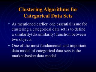
21. Review of existing algorithms K-modes • This algorithm is built on the idea of K-means algorithm. • It demands the number of clusters. • Partition is sensitive to the input order. • Computational Complexity O(n)

22. AutoClass Algorithm This algorithm can cluster both categorical and numeric data types. 1. It utilizes the EM algorithm. 2. It searches the optimal number of clusters 3. EM algorithm is known to have slow convergence. 4. The computational complexity is O(n).

23. Categorical Sample Space • Assume that the data set is stored in a n*p matrix, where n is the number of observations and p the number of categorical variables. • The sample space consists of all possible combinations generated by p variables. • The sample space is discrete and has no natural origin.

24. Hamming Distance and CD vector • Hamming distance measures the number of different attributes between two categorical variables. • Hamming Distance has been used in clustering categorical data in algorithms similar to K-modes. • We construct Categorical Distance (CD) vector to project the sample space into 1-dimesional space.

25. Example of a CD vector

26. More on CD vector • The dense region of the CD vector is NOT necessarily a cluster! • The length of the CD vector is p. • We can construct many CD vectors on one data set by choosing different “origin”.

27. How to detect a cluster ? • The CD vector shows some clustering pattern. But are they statistically significant? • Statistical Hypothesis Testing: Null Hypothesis: Uniformly distributed. Alternative: Not uniformly distributed. • We call the expected CD vector under the null Uniform CD vector (UCD).

28. UCD: Expected CD vector under Null.

29. CD Vector UCD Vector

30. How to compare these 2 vectors? • One is the observed CD vector. • The other is the expected CD vector under null hypothesis. • Chi-square is the most natural tool to test the null hypothesis based on these two vectors. • However clustering patterns are all local features. Thus we are not interested in a comparison at a global level.

31. Modified Chi-square Test The modified Chi-square is defined as:

32. Choice of C and Radius of a Cluster

33. CD Algorithm • Find a cluster center; • Construct the CD vector given the current center ; • Perform modified Chi-square test; • If we reject the null, then determine the radius of the current cluster; • Extract the cluster • Repeat until we do not reject the null.

34. Numerical Comparison with K-mode and AutoClass CDAutoClassK-mode No. of Clusters 4 4 [3] [4] [5] _____________________________________________________ Classi. Rates 100% 100% 75% 84% 82% “Variations” 0% 0% 6% 15% 10% Inform. Gain 100% 100% 67% 84% 93% “Variations” 0% 0% 10% 15% 11% _____________________________________________________ Soybean Data: n=47 and p=35. No of clusters=4.

35. Numerical Comparison with K-mode and AutoClass CDAutoClassK-mode No. of Clusters 7 3 [6] [7] [8] _____________________________________________________ Classi. Rates 95% 73% 74% 72% 71% “Variations” 0% 0% 6% 15% 10% Inform. Gain 92% 60% 75% 79% 81% “Variations” 0% 0% 7% 6% 6% _____________________________________________________ Zoo Data: n=101 and p=16. No of clusters=7.

36. Run Times Comparison K-modes CD ____________________________________ Soybean Average 0.0653 0.0496 S.D 0.0029 0.0010 Zoo Data Average 0.0139 0.0022 S.D 0.0018 0.0001 ____________________________________ Note that AutoClass requires human intervention.

37. Computational Complexity • The upper bound of the computational complexity of our algorithm is O(kpn) • Note that the sample size shrinks if the CD algorithm detects a cluster • It is less computational intensive than K-modes and AutoClass since both have complexity of O(akpn) where a>1.

38. Conclusion • Our algorithm requires no convergence criterion. • It automatically estimate the number of clusters. It does not demand or search for the true number of clusters. • The sample size is reduced after one detected cluster is extracted. • The computational complexity of our algorithm is bounded by O(n).

39. Future Work • Clustering functional data. • Clustering mixed data, continuous and categorical data at the same time. • Clustering data with spatial and temporal structure. • Develop parallel computing algorithms for our methods.

40. Reference: Zhang, P, Wang, X. and Song, P. (2007) Clustering Categorical Data Based on Distance Vectors. JASA.

41. Software Download • http://math.yorku.ca/~stevenw • Please go to Software section and you can download the program. • We are also in the process of developing a C program for both methods.