3.5 WIND LOADS 3.5.1 Wind phenomenology Wind speed is experienced essentially at two different time scales:
3.5 WIND LOADS 3.5.1 Wind phenomenology Wind speed is experienced essentially at two different time scales:

3.5 WIND LOADS 3.5.1 Wind phenomenology Wind speed is experienced essentially at two different time scales:
E N D
Presentation Transcript
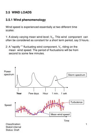
3.5 WIND LOADS3.5.1 Wind phenomenology Wind speed is experienced essentially at two different time scales: 1: A slowly varying mean wind level; Vm. This wind component can often be considered as constant for a short term period, say 3 hours. 2: A ”rapidly ”” fluctuating wind component, Vt, riding on the mean wind speed. The period of fluctuations will be from second to some few minutes. Powerspectrum Storm spectrum Year Few days Hour 1 min. 1 sek Turbulence Speed Mean wind speed Time
At a given point, the resulting wind speed can be written:V(t) = Vm(t) + Vt(t) The mean wind speed is typically the largest. Terrain roughness govern the ratio. The ratio between standarddeviation of Vt and Vm is called turbulence intencity. Typical turbulence intencity over ocean with storm waves is about 0.12. The wind speed varies with height, see eq(1a – 1d) in Statoil metocean report. For engineering purposes, the mean wind speed is described by a distribution function often close to a Rayleighdistribution. The mean direction is described by a probabilitymass function for direction sectors (often) of 30 deg. width. The mean wind speed corresponds to a given length of averaging. Standard meteorological averaging is 10 min.., in design the length of averaging is often taken to be 1 hour. Wind speed will increase with decreasing length of averaging.The ration between a 15sek average and a 1-hour average 10m above sea level is 1.37, see table in Statoil report for other examples. Example of a wind description for design purposes is shownby Statoil Metocean report.
For structures or structural components where the turbulentwind may cause a dynamic behaviour, the frequency spectrumfor wind speed is given by Eq. (2a and 2b) of Statoil Report orNorsok N-003. This wind spectrum is deduced from wind measurements atFrøya. The turbulent wind is not fully correlated over the size of structures. Coherence spectrum between two points are given in Statoil report or Norsok N-003. The loads on structures not exposed to dynamic behaviour can be calculated considering the wind as static:If structural dimensions are less than 50m, 3s gust should beused.If structures are larger, 15s gust can be used. For structures which are exposed to simultaneous actionsfrom wind and waves, and where the wave loading is dominating, the length of averaging of wind gust may be taken to be 1 minute. Check with coming editions of Norsok forpossible changes.
3.5.3 Wind forcesThe wind force is proportinal to the wind speed squared: F = k * (Vm + Vt)2 = Vm2 + 2VmVt + Vt2 =(ca) Vm2 +2VmVtThe mean wind gives a constant force on the structure, while the turbulent wind yields a force proportional the theturbulent wind speed. Practical problems:Offset and mooring line forces for ships and floating platforms.The natural periods of the surge, sway and yaw are oftenin the order of 1-2 minute, i.e. a period band where the wind frequncy spectrum has a considerable power density.For this sort of problem, a dynamic analysis has to be carried out involving the wind power spectrum. Wind loading on flare towers and drilling towers. A quasi-static analysis is often possible accounting for some dynamics by a proper dynamic amplification factor. The wind loading on complicated structures are determinedby means of tests in wind tunel. Remember that in all cases mentioned above, one will alsohave to include the simultaneous affect of waves.
The static wind force on a structural member or surface acting normal to the member or surface is given by:FW = ½ C A V2 sinC – shape coefficient, see DNV 30.5 – density of air (= 1.225 kg/m3 for dry air)A – projected area of member normal to force direction – angle between wind and axis of the exposed member For the wind load of a plane truss, the load can be calculated by using A as the enclosed area of truss if aneffective shape parameter is used, C=Ce, and the transparancy of the truss is accounted for by multiplyingthe area with the solidity ratio Ce is found in DNV 30.5. If more than one member or truss are located behind eachother, shielding effect can be accounte for by multiplyingloads given above by the shielding factor,. Values for are given in DNV 30.5. Regarding the shape coefficicent, it is recommended that DNV 30.5 or an similar reference are consulted. NB: For structural sides not facing the wind, a considerablesuction force can occurr, see Fig. 3.14 b in kompendium,Moan (2004).
If structure or structural component can be exposed to windinduced dynamics, the variability of the wind force is to be accounted for:FW(t,z) = ½ C A (Vm(z)2 + 2* Vm(z)*Vt(z,t)) * sin It is seen that load is linear with respect to wind speed (since Vt2 term is neglected). If the wind induced response is linearfunction of load, the wind response may be obtained using frequency domain analysis, i.e. the cross spectral density for the dynamic wind load is multiplied by response transferfunction in order to obtain response spectra for dynamicwind induced response. Alternatively, wind histories for a number of load points maybe simulated from wind spectrum and corresponding timehistories for the response found by solving the equation of motion in time domain. The total extreme wind induced response can be found by:F3h-max (Vm) = Fm + g * (Vm)g – extreme value factor for 3-hour maximum dyn. response – standard deviation of wind response under consideration
Vortex Induced Vibrations (brief introduction)Vortex shedding frequency in steady flow is given by:f = St * V/D St is the Strouhal number, V is wind speed and D is structuraldiameter. A critical velocity is defined as the velocity giving vortex shedding frequencies equal to the natural frequency of the structural member:VC = 1/St * fN * DfN – natural frequency of structural member. St is a function of the Reynolds number, Re = VD/, where is the kinematic viscosity of air, (= 1.45*10-5 m2/s at 15oand standard atmospheric pressure. St is given in Fig. 7.1 in DNV 30.5. A state of quasi-resonant vibriations of a member may take place if wind velocity is in the range:K1*VC < V < K2*VC If possible, one should require: VC > 1/K1 *VmaxNot always possible and maybe unnecessary strict criterium.
3.6 Wave and Current loadsWater levels: Maximum still water level Positivestorm surge Highest astronomical tide (HAT) Mean still water level Tidalrange Lowest astronomical tide (LAT) Negativestorm surge Minimum still water level Classification of structures* hydrodynamic transparent (slender structures, Morison loading)* hydrodynamic compact (large volume structures, diffraction analysis)
When to account for which effects? Bølger og strøm viktig Bølger viktigst
3.6.2 Current velocity fieldFor most design work, current profiles (speed versus depth) are established from current measurements. Measurements are typically made at a number of depths. Upto now extremes are typically estimated for each depth separately. Linear interpolation between depths. It is likely that such profiles are concervative for most cases,but not necessarily for all. 10-1 – design profile Presently work is going on regarding developing more adequat design profile:* Current is described as a sum of empirical orthogonalfunctions. * Family of profiles with 10-2 speed at one depth and associated values at other depths.
Current components:* Tidal current.* Background current.* Wind driven current* Meanders or vortex current If data are not avvailable, current field may be taken as the sum of the tidal current (constant through water column)and the wind driven current (= 1-2% of mean wind speed atthe surface decaying linearly to zero at about 50m. In connection with loads on structures, the current isconsidered as a slowly varying phenomenon, i.e. the current speed is kept constant for a short term sea state. Typical surface current speed North Sea (no eddies present): 10-1 - current: 1m/s
3.6.3 Waves and descrition of wavesThe sea surface is of an irregular nature, but it can to a first appoximation be written as a sum of sinusoidal with different amplitude, different frequency, (different direction)and different phase. For practical application, the long term variation of the seasurface elevation process is consider as i piecewisestationary (and homogeneous) stochastic process (field).If the sea surface elevation can be modelled as a Gaussianprocess, each stationary sea state is in a statistical sense completely characterized by the directional wave spectrum:Sh(f, ) = sh(f)*d() Spreading function Frequency Spectrum Several models are proposed for the frequency spectrum:* ISSC (Generalized Pierson Moskowitz, fully developedwind sea)* JONSWAP (pure wind sea, may be growing)* Torsethaugen (combined sea, wind sea + swell)Common for all models is that they are parameterized interms of significant wave height, hs, and spectral peak period, tp.
Long term modelling of sea states In view of what is said above, one can conclude that a short term sea state is for practical purposes described in terms of significant wave height, spectral peak period and direction of propagation. The long term description of wave conditions can be doneby establishing a joint probability density function forHs, Tp and :fHs,Tp,(h,t,) = f Hs,Tp|(h,t|)*f() where: approximated by prob. mass function fHs,Tp(h,t) = fHs(h) * fTp|Hs(t|h) Log-normal or Weibullfitted to data for eachhs - class 3-p Weibull or LonoWe Fitted to available data
Short term modelling of sea states It is most common to use long crested sea. This may benon-conservative for ships heading into sea with respect toassess ship rolling. Select spectral model in view of problem to be considered.
Torsethaugen versus JONSWAP For a further illustration of how to descibe sea states in short and long term for practical applications, see e.g. the Statoil Metocean report.
Prediction of extreme sea states and wavesSea statesVarious approaches are used:* All sea state approach (based on modelling Hs and Tp for all 3-hour stationary sea states. Most commonly adopted approach in Norwegian waters* Peak over threshold approach (based on modellingmerely storm peak characteristics. Most common in areas of a mixed population wave climate, i.e. a distinctdifference between normal conditions and stom conditions.) In the following we will stay with the first approach:The number of 3-hour sea states per year is 2920 if all directions and seasons are pooled together: The 10-2 – probability significant wave height is then estimated by:1 – FHs(h_10-2) = 1/ (2920*100) Corresponding peak period:
If structural response is rather sensitive to the peakperiod, it is not necessarily the highest 10-2 sea statethat is the most critical. In order to cover these needs lines of hs and tp corresponding to a constant probabilityof exceedance are often provided: It will be indicated later how such a contour can be used for design load calculations.
Prediction of extreme individual waves For a number of response problems, the sea surface process can for practical applications be modelled as a Gaussian process. If the purpose of the assessment is to predict accurate extreme individual waves, this should not be done.Regarding crest height, a proper model is the distribution recommended by Forristall. Where: Short term extreme value: FC(c3hmax) = 1- FC(c3hmax) = 1/m3h No. of crest heightsin 3 hours. Characteristic maximum
Forristall model is based on fitting a Weibull model to a hugenumber of simulations of second order surfaces for various conditions. Regarding wave heights, the model proposed by Arvid Næss(1985) is recommended. This model is a bandwidth correctedRayleigh distribution.
Regarding a prediction of long term extremes, a long term analysis should be carried out: The 10_2 crest height is then given by:1- FX3hour (x_10-2) = 1/ = 10-2 / 2920 Alternatively, one may use the environmental contour principle. This includes the following steps:a) Find worst sea state along 10-2 contour line.b) Establish the distribution function for the 3-hour maximumcrest height. c) An estimate for the 10-2 crest height is obtained by adopting the 90-percentile of this distribution.
A so far unsolved question regarding waves, is the possible existence of freak waves. (From: BBC Horizon)
What can be the problem if freak waves exist? The above scenario is completely unacceptable, In particular for manned structures, it is therefore a good idea to ensure a reasonable robustness against unexpectedly large crest heights. For a given site freak waves if they exist are most probably so rare that they will not effect our 10-2 and 10-4 predictions. But if a possible freak wave mechanism will occur more frequently in sea statesbeyond thos thatr are observed so far, this conclusionmay have to be adjusted.
Wave loads For the purpose ofthis course, we willassume these loads to belinear and characterized by a transfer function. In the following we will focus on thesetype of loads.
3.6.5 Large volume structuresFixed platformsMost important load is wave frequency load. The load is Most often approximated very well by a linear potential theory. The loadis typically described by the transferfunction or response amplitude operator:H() = x()/()where () is a harmonic wave, () = 0exp(-it) and x() is the response due to this harmonic wave, x() = x0 exp(-i(t+)) H() = x0/h0 exp(-i ) = |H()| exp(-i)A closed for solution for H() can be found for some few cases, most of the time H() is found for the various frequencies using numerical methods. In addition to the wave frequency load, there will also be a slowly varying force on the platform corresponding todifference frequencies and a high frequency load corresponding to the sum frequencies. These are much lower than the wave frequency load, but the high frequencyload may for some structures hit the largest natural period and thus cause som resonant response. This is referred to as ringing.
Floating structuresThe same can be said as for the fixed platforms. However,the slowly varying load can now hit the natural period of the horisontal modes of motion and cause rather large offset motiona and mooring line forces. For a TLP the sum frequency term can hit the natural period of the vertical modes of motions Response calculations Select a sea state, hs and tp. The wave spectrum is then known. As the transfer function has been calculated, the response spectrum is given by:sx() = | H()|2 s() The variance and zero-up-crossing frequency can be found from the spectral moments, m0 and m2. THe response process can often be assumed to be Gaussian,this means that the global maxima of the response processis desribed by the Rayleigh distribution. FXmax | Hs,Tp (x | hs,tp) = 1 – exp(-0.5 (x / X)2), X = X(h, tp)
Long term distribution of Xmax is given by: 10-2 response maximum is given by: Alternatively, the environmental contour approach can beadopted. However, for linear systems one may just as well do a classical long term analysis as indicated above.