TinyOS and Sensor Network Applications
Explore how TinyOS facilitates analog and digital data interface for sensor network applications, including magnetometer usage and efficient tree construction processes. Learn about optimizing traffic light controllers, enhancing parking lot operations, and implementing accurate tree routing procedures in sensor networks.


TinyOS and Sensor Network Applications
E N D
Presentation Transcript
TinyOS and Sensor Network Applications Sinem Coleri WOW - 01/18/2002
Outline • TinyOS • Analog Data Interface • Magnetometer • Digital Data Interface • Tree Construction • Sensor Network Applications • Parking Lot • Traffic Light Controller
ADIE ADC Multiplexer Select Bits (2 1 0) ADC Control Register ADC7 ADEN ADSC ADIF ADC6 ADC5 ADC4 ADC9..0 8-channel MUX ADC Data Register A/D converter ADC3 ADC2 ADC1 ADC0 Analog Data Source2 Analog Data Source1 Analog Data Interface • 8-channel analog multiplexer • Allows to connect more than one analog sensor • A/D Converter • Converts analog input voltage to 10-bit digital value • Operates in single conversion mode • Conversion initiated by user
ADIE ADC Multiplexer Select Bits (2 1 0) ADC Control Register ADC7 ADEN ADSC ADIF ADC6 ADC5 ADC4 ADC9..0 8-channel MUX ADC Data Register A/D converter ADC3 ADC2 ADC1 ADC0 Analog Data Source2 Analog Data Source1 Analog Data Interface • AIM: • sample a specific analog data source • STEPS: • Call command ADC_GET_DATA with argument of channel number • Continue execution or sleep • Take digital data while executing interrupt handler upon receiving ADC interrupt
ADIE ADC Multiplexer Select Bits (2 1 0) ADC Control Register ADC7 ADEN ADSC ADIF ADC6 ADC5 ADC4 ADC9..0 8-channel MUX ADC Data Register A/D converter ADC3 ADC2 ADC1 ADC0 Analog Data Interface • ADMUX bits 2..0 • Used to select which analog input is connected to ADC • Specified as an argument in command ADC_GET_DATA • ADEN-ADC Enable • Used to turn ADC on and off • Set in command ADC_GET_DATA and cleared in interrupt handler to save power
ADIE ADC Multiplexer Select Bits (2 1 0) ADC Control Register ADC7 ADEN ADSC ADIF ADC6 ADC5 ADC4 ADC9..0 8-channel MUX ADC Data Register A/D converter ADC3 ADC2 ADC1 ADC0 Analog Data Interface • ADSC-ADC Start Conversion • Used to start conversion when set and cleared by hardware at the end of conversion • Set in command ADC_GET_DATA • ADIE-ADC Interrupt Enable • Used to enable ADC interrupt • ADIF-ADC Interrupt Flag • Used to learn the end of conversion and register update • Set by hardware • Interrupt handler executed if both ADIE and global interrupt enable bits are set when ADIF set
Vcc R R+R Amplifier R R+R Magnetometer Function: • To detect magnetic materials, such as cars, from the change in the earth’s magnetic field Magnetometer circuit: • Magneto-resistive elements configured in an H-bridge • Software controlled nulling in order not to saturate amplifier
Magnetometer Vertical lines mark the start/stop points of the mote's determination that a vehicle is present. Green trace is the raw signal. Yellow is low-pass filtered signal. Red is high-pass filtered yellow.
Magnetometer • In high way or for the traffic light controller, • The previous algorithm only detects cars with speeds in a specific interval. • Higher speed cars missed while passing through high-pass filter in removing sampling noise • Lower speed cars missed while passing through high pass filter in detecting the change in the field • Solution • Adjust the sampling rate high enough to detect highest speed cars • Consider the absolute magnetic field to detect lower speed cars
Magnetometer • In parking lot, • Nodes can make incorrect decisions • Magnetic field changed by • Car passing between sensors looking for a place or going away • Car going to the adjacent slot • Once node makes a mistake, it cannot correct on the next sample since it only check the filter output • Solution • Consider the absolute magnetic field • Procedure: • Keep the DC offset value and ADC reading value when there is no car • Compare current DC offset value and ADC reading value to the original one to determine the car • Possible questions: • The magnetic field change from the car above the sensor may not be higher compared to combined effect from the adjacent cars • Can we use other sensors, such as light sensor?
Digital Data Interface • No example dealing with digital data • I2C protocol can be used to connect more than one digital sensor • Main processor as master, digital sensors as slaves • Communication between master and one of the slaves • Master starts transmission • Master selects the slave to communicate by a 8-bit address and the direction
Tree Construction Each data packet destination is Base Station Nodes only need to determine next hop to reach BS from the shortest path Set of optimal routes from all sources to a given destination form a tree routed at destination AIM: to form a tree routed at Base Station and consisting of the optimal routes from all sensor nodes to BS
2 1 3 2 1 Tree Construction Base Station • Periodically broadcasts ROUTE_UPDATE packet • Source address = Base ID, num_of_hops = 0 Sensor Node • Keeps its parent and its depth in the tree • When it takes ROUTE_UPDATE packet • If no update received for an expiration time or num_of_hops < depth • Update parent = source address, depth = num_of_hops+1 • Broadcast ROUTE_UPDATE with source address = own address, num_of_hops = depth 0 Base
3 2 5 0 Base 4 1 Tree Construction Problem in TinyOS: • No queue -> Drop packet if transmitting another packet • Connectivity may be lost • If 2 and 4 drop packets, then 3 and 5 will be disconnected • Nodes may choose parent over a longer path • If 2 drops packet but 4 does not drop packet, 3 will be connected to BS over 3 hops instead of 2 Solution: • Queued tree construction: • Each node puts route packet to the head of the queue • Reason: • Packets with higher num_of_hop field arrive earlier -> increase in number of route packets broadcasted • If queue is long in 2 and is short in 1 and 4, packet from 4 come earlier
Parking Lot: Scenario #1 • Suppose • Sensor nodes are located as in the figure below • Each sensor node has a different ID • Each sensor node location is known by BS BS
Parking Lot: Scenario #1 • Tree construction same as explained before: • BS broadcasts route update packet • Each sensor node determines its parent from the route update packets • BS determines the location of free spaces from • Data packet including data and ID of source node • Location information mapping ID to location BS
Parking Lot: Scenario #2 • Suppose • Sensor nodes are located as in the figure below • Each sensor node has a different ID • Sensor node locations are not known by BS BS
Parking Lot: Scenario #2 • Determining the location of the nodes based on RF communication: • Assumptions: • Idealized radio model • Perfect spherical range of d • Identical transmission range for all radios • Knowledge of the location of the two second-hop nodes d d BS
#15 #14 #13 #12 #11 #10 #9 #8 #2 #4 #5 #6 #7 BS #3 Parking Lot: Scenario #2 • Observations: • The nodes on the same diagonal have the same depth in tree • Each node takes either one or two route update packets with min. num_of_hop field • Algorithm: • Each node keeps the sources of the route update packets with min. num_of_hop field as parents but choose one for routing • Each node include its depth and its parents in data packet • BS determines the location of nodes starting from the nodes in #3 diagonal
Parking Lot: Scenario #3 • Suppose • Sensor nodes are located as in the figure below • Sensor nodes are not assigned an ID • Sensor node locations are not known by BS BS
(7,0) (8,0) (9,0) (10,0) (11,0) (12,0) (13,0) (14,0) (6,1) (7,1) (8,1) (9,1) (10,1) (11,1) (12,1) (13,1) (5,2) (6,2) (7,2) (8,2) (9,2) (10,2) (11,2) (12,2) (4,3) (5,3) (6,3) (7,3) (8,3) (9,3) (10,3) (11,3) (3,4) (4,4) (5,4) (6,4) (7,4) (8,4) (9,4) (10,4) (2,5) (3,5) (4,5) (5,5) (6,5) (7,5) (8,5) (9,5) (1,6) (2,6) (3,6) (4,6) (5,6) (6,6) (7,6) (8,6) (0,7) (1,7) (2,7) (3,7) (4,7) (5,7) (6,7) (7,7) BS Parking Lot: Scenario #3 • IDEA: • Each node assigns itself an address of type (depth, offset) from the route update packets received from neighbors • ASSUMPTION: • Two second-hop nodes((1,6) and (1,7)) know their address • ALGORITHM: • Wait for some constant time for other packets after receiving route update packet • Keep (depth,offset) of minimum depth packets • Assign its (depth,offset) by ASSIGN_ADDRESS procedure • Send route update and data packets with this (depth,offset) address
(7,0) (8,0) (9,0) (10,0) (11,0) (12,0) (13,0) (14,0) (6,1) (7,1) (8,1) (9,1) (10,1) (11,1) (12,1) (13,1) (5,2) (6,2) (7,2) (8,2) (9,2) (10,2) (11,2) (12,2) (4,3) (5,3) (6,3) (7,3) (8,3) (9,3) (10,3) (11,3) (3,4) (4,4) (5,4) (6,4) (7,4) (8,4) (9,4) (10,4) (2,5) (3,5) (4,5) (5,5) (6,5) (7,5) (8,5) (9,5) (1,6) (2,6) (3,6) (4,6) (5,6) (6,6) (7,6) (8,6) (0,7) (1,7) (2,7) (3,7) (4,7) (5,7) (6,7) (7,7) BS Parking Lot: Scenario #3 • ASSIGN_ADDRESS Procedure: • Assign (minimum depth + 1) to depth • If number of sources with min. depth is 1 • If its depth + its offset = 7 • Assign (offset – 1) to offset • Else if its offset is 7 • Assign 7 to offset • Else(means that it missed one packet) • Assign either (offset) or (offset – 1) to offset • Else if number of sources with min. depth is 2 • Assign minimum of their offset to offset • This can easily be generalized to any dimension
Parking Lot: Scenario #3 (7,0) (8,0) (9,0) (10,0) (11,0) (12,0) (13,0) (14,0) NEXT STEP-> CLUSTERING GOAL: • To conserve power • Include data aggregation into the scheme • To distribute power consumption • Prevent nodes closest to BS from routing a large number of data packets to BS • To satisfy real-time delivery requirements ALGORITHM: • Route update packets include cluster width and length • Nodes find their coordinates wrt. cluster head by choosing the bottom left corner as cluster head (6,1) (7,1) (8,1) (9,1) (10,1) (11,1) (12,1) (13,1) (5,2) (6,2) (7,2) (8,2) (9,2) (10,2) (11,2) (12,2) (4,3) (5,3) (6,3) (7,3) (8,3) (9,3) (10,3) (11,3) (3,4) (4,4) (5,4) (6,4) (7,4) (8,4) (9,4) (10,4) (2,5) (3,5) (4,5) (5,5) (6,5) (7,5) (8,5) (9,5) (1,6) (2,6) (3,6) (4,6) (5,6) (6,6) (7,6) (8,6) (0,7) (1,7) (2,7) (3,7) (4,7) (5,7) (6,7) (7,7) BS
Parking Lot: Scenario #3 (7,0) (8,0) (9,0) (10,0) (11,0) (12,0) (13,0) (14,0) EXAMPLE: Width=4, length=4 (x,y)=(depth,offset) (xh,yh)=coordinates wrt.cluster head • xh = mod(x+y-7,width) = mod(x+y-7,4) • yh = mod(7-y,length) = mod(7-y,4) Distance to cluster head in terms of number of hops = xh + yh (6,1) (7,1) (8,1) (9,1) (10,1) (11,1) (12,1) (13,1) (5,2) (6,2) (7,2) (8,2) (9,2) (10,2) (11,2) (12,2) (4,3) (5,3) (6,3) (7,3) (8,3) (9,3) (10,3) (11,3) (3,4) (4,4) (5,4) (6,4) (7,4) (8,4) (9,4) (10,4) (2,5) (3,5) (4,5) (5,5) (6,5) (7,5) (8,5) (9,5) (1,6) (2,6) (3,6) (4,6) (5,6) (6,6) (7,6) (8,6) (0,7) (1,7) (2,7) (3,7) (4,7) (5,7) (6,7) (7,7) BS
Parking Lot: Scenario #3 (7,0) (8,0) (9,0) (10,0) (11,0) (12,0) (13,0) (14,0) Hierarchy schemes: 1) AIM: • To conserve power by aggregating data at cluster head ALGORITHM: • Each node in the cluster • Sends their data packet to cluster head • Forwards others’ packet to cluster head • Cluster head • Does data aggregation for the data packets not marked as “aggregated” and mark it as ‘aggregated” • Sends the aggregated data packet to one of its parents • Forwards data packets marked as “aggregated” to one of its parents (6,1) (7,1) (8,1) (9,1) (10,1) (11,1) (12,1) (13,1) (5,2) (6,2) (7,2) (8,2) (9,2) (10,2) (11,2) (12,2) (4,3) (5,3) (6,3) (7,3) (8,3) (9,3) (10,3) (11,3) (3,4) (4,4) (5,4) (6,4) (7,4) (8,4) (9,4) (10,4) (2,5) (3,5) (4,5) (5,5) (6,5) (7,5) (8,5) (9,5) (1,6) (2,6) (3,6) (4,6) (5,6) (6,6) (7,6) (8,6) (0,7) (1,7) (2,7) (3,7) (4,7) (5,7) (6,7) (7,7) BS
(7,0) (8,0) (9,0) (10,0) (11,0) (12,0) (13,0) (14,0) (6,1) (7,1) (8,1) (9,1) (10,1) (11,1) (12,1) (13,1) (5,2) (6,2) (7,2) (8,2) (9,2) (10,2) (11,2) (12,2) (4,3) (5,3) (6,3) (7,3) (8,3) (9,3) (10,3) (11,3) (3,4) (4,4) (5,4) (6,4) (7,4) (8,4) (9,4) (10,4) (2,5) (3,5) (4,5) (5,5) (6,5) (7,5) (8,5) (9,5) (1,6) (2,6) (3,6) (4,6) (5,6) (6,6) (7,6) (8,6) (0,7) (1,7) (2,7) (3,7) (4,7) (5,7) (6,7) (7,7) Parking Lot: Scenario #3 Hierarchy schemes: 2) AIM: • To conserve power by data aggregation(same as 1) • To distribute power consumption by allowing cluster heads to send from one cluster to the other • To satisfy real-time delivery requirements ALGORITHM: • Each node in the cluster(same as 1) • Sends and forwards data packets to cluster head • Cluster head • Does data aggregation for the data packets • Sends the aggregated data packet over cluster distance • Cluster head can change inside the cluster in order to avoid cluster heads from dying BS
(7,0) (8,0) (9,0) (10,0) (11,0) (12,0) (13,0) (14,0) (6,1) (7,1) (8,1) (9,1) (10,1) (11,1) (12,1) (13,1) (5,2) (6,2) (7,2) (8,2) (9,2) (10,2) (11,2) (12,2) (4,3) (5,3) (6,3) (7,3) (8,3) (9,3) (10,3) (11,3) (3,4) (4,4) (5,4) (6,4) (7,4) (8,4) (9,4) (10,4) (2,5) (3,5) (4,5) (5,5) (6,5) (7,5) (8,5) (9,5) (1,6) (2,6) (3,6) (4,6) (5,6) (6,6) (7,6) (8,6) (0,7) (1,7) (2,7) (3,7) (4,7) (5,7) (6,7) (7,7) Parking Lot: Scenario #3 Hierarchy schemes: 3) AIM: • To conserve power by data aggregation(same as 1) ALGORITHM: • Each node in the cluster • Waits proportional to (max number of hops to cluster head – distance to cluster head) • Aggregates its own data with the received data • Sends the aggregated data packet to cluster head • Cluster head • Does data aggregation for the incoming packets • Sends the aggregated data packet either as a normal packet or over cluster distance BS
Conclusion • TinyOS • Analog Data Interface • How to get data, conserve energy and connect more than one analog data source • Magnetometer • How it works, how to process the data • Digital Data Interface • How to connect more than one digital data source • Tree Construction • How TinyOS constructs tree, how to make it more efficient • Sensor Network Applications • Parking Lot • How to estimate the location of nodes based on RF communication • How to send data to Base Station • Traffic Light Controller • How to send data to Base Station • How to adjust the duration of traffic lights