Download
1 / 25
270 likes | 513 Vues
Modeling & Control of Magnetic Levitation System. By Marwan K. Abbadi Advisor: Dr. W. Anakwa Date: March 11th 2003. Outline. Overview Project Description - Objective - Functional Description - System Block diagram - Mathematical Model - Software Flowchart

E N D
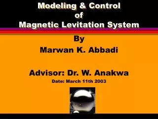
Modeling & Control of Magnetic Levitation System By Marwan K. Abbadi Advisor: Dr. W. Anakwa Date: March 11th 2003
Outline • Overview • Project Description - Objective - Functional Description - System Block diagram - Mathematical Model - Software Flowchart • Project Status • Updated timeline • References
Overview • Magnetic Levitation Systems • Definition • Nature:non-linear and open-loop unstable • Objective of the project: • Modeling:Derive mathematical equations that describe the system dynamics and validate the model experimentally • Controller:Design stabilizing controller and implement the controller equations on an 8051 micro-controller to suspend the ball at a desired position
Functional Description • Inputs: • Desired vertical position of the ball • Disturbances could be • Externally: Varying the disturbance input to the plant • Internally: From the internal system such as power supply fluctuation • Output: • Actual ball position • Feedback: • Analog signal corresponding to the ball position
System Layout Plant 8051UC HW + SWController Ball position: 22.5 mm ‘C’= Restart
Mathematical Model • There are two sets of equations that govern the dynamics of the system: • Electrical equation- relates the ball’s suspension X with the input voltage e. Obtaining KVL around circuit e = R. i+ L.di/dt - (Lo. x0.i/x^2)dx/dt (1)
Electromagnetic force EF= C (i/x)2 Gravitation force GF = m*g Mathematical Model • Mechanical equation- relates the resultant force applied to the ball with the distance from the electromagnet From the force diagram F= GF- EF = m.g - C (i/x)2 (2)
Mathematical Model • Linearization of the mathematical model To develop a linear model of the plant about a specified operating point Xo. • Method of linearization Use of Taylor series expansion to linearize the model about an operating point Fmag= C(I/x)^2 Delta F = 2C{ io/Xo2 delta I - io^2/Xo^3 delta X) Where Xo, io are the parameters at the linearized operating point
Mathematical Model(Experimental determination of Variables) • Magnetic force constant - Plant is highly sensitive to temperature. - Several attempts were taken to calculate the plant’s constant. Method: - An analog controller was connected to stabilize the plant. - The gain of the controller was adjusted till the ball slightly suspended upwards. The ball was assumed to be at mechanical equilibrium(F=0) - The position of the ball and current flowing through coil were recorded and substituted in the previous equation. - C was found to be 1.477x10^-4 N.m2.A-2
Mathematical Model(Experimental determination of Variables) • Coil inductance vs. Ball distance from electromagnet • Exhibits a non-linear relationship • The coil inductance was measured at different ball positions. • Found to be fairly constant about the operating range of 18 to 27mm. (Full-range inductance variation=210uH) • After linearization, the inductance was set to be constant( = 296.74mH)
Mathematical Model(Experimental determination of Variables) • Coil inductance vs. Ball distance from the electromagnet
Mathematical Model(Experimental determination of Variables) • Calibrating the sensor • Highly sensitive to opaque objects Method of calibration: • A transparent tube-calibrator was used to place the ball at different positions. • Assumption taken that the calibrator’s interference is small. This assumption had to be verified experimentally by removing the ball and placing the tube-calibrator between the sensor plates. • The relationship between the position of the ball and the sensor’s voltage was found to be linear as expected.
Mathematical Model(Experimental determination of Variables) Sensor voltage vs. Ball distance about the operating point
Mathematical Model(Experimental determination of Variables) • Combining all the equations and substituting the measured constants, the overall plant’s transfer function was obtained analytically. X(s) 0.4838 -------=------------------------------------------------------------------------------ E(S) 0.006232 s^3 + 0.4386 s^2 - 5.29 s - 372.3
Mathematical Model(Experimental determination of Variables) • Root locus sketch of the plants’ poles (Notice the plant’s zeroes are located @ infinity)
Mathematical Model(Experimental determination of Variables) • Step response of the open-loop transfer function.
Mathematical Model(Experimental determination of Variables) • Next step in the mathematical modeling is verifying the model experimentally, which is the current task being performed. Closed-loop frequency response data were measured and recorded for graphical analysis. More data needs to be measured to finalize the modeling, and obtain the actual transfer function of the plant.
Actual Error Signal Position, Xo E= Xi-Xo Desired position Xi Multiplexed 8-bit A/D Converter Control Algorithm LCD Sampled u(k)=f [e(k)] displaying desired and error Signal actual ball position e(k) u(k) 8-bit D/A u(t) Converter Software Flowchart
Software • 8051 micro-controller • Developed assembly language modules for sampling an input signal via the A/D converter and producing it at the D/A converter. User-interface module is fully completed. • Managed to code a software skeleton for implementing a hypothetical digital filter (code modification will be done later for the actual filter). • Verified the digital filter code by running it on the simulator, but was unsuccessful with real-time signals. • Task not fully accomplished.
Software • Signal sampled through the A/D and produced via the D/A converter.(Freq=7Khz)
Updated Project timeline • March • Finalize the modeling phase and obtain the validated transfer function of the plant. • Design a stabilizing controller and verify its response using Matlab • Adjust the controller to account for stability, noise rejection, phase margin and overshoot specifications.
Updated Project timeline • April • Design hardware components required by the controller. • Finish coding and debugging the digital filter. • Test the overall software and verify its operation. • Interface the hardware and software and verify the overall system performance.
Updated Project timeline • May • Continue debugging the overall system.
References • Barie and Chiason, International Journal of System Sciences, 1996, vol 27 • D’Azzo and Houpis, Linear control system analysis and design: Conventional and Modern. • Dempsey, Bradley Univ.EE431-EE432 Lecture notes, 2003. • Grabbe, Ramo and Wooldridge, Handbook of automation, computation and control, vol.1 • Wong, IEEE Trans. on Education, 1986, vol. E29#4.
The End http://cegt201.bradley.edu/projects/proj2003/maglev Questions Comments Thank you