Global Earthquake Data : Local e.q. catalogs tend to have problems, esp. missing data.
360 likes | 535 Vues
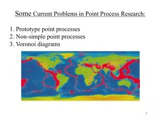
Some Current Problems in Point Process Research: 1. Prototype point processes 2. Non-simple point processes 3. Voronoi diagrams. Global Earthquake Data : Local e.q. catalogs tend to have problems, esp. missing data. 1977: Harvard (global) catalog created.

Global Earthquake Data : Local e.q. catalogs tend to have problems, esp. missing data.
E N D
Presentation Transcript
Some Current Problems in Point Process Research:1. Prototype point processes 2. Non-simple point processes3. Voronoi diagrams
Global Earthquake Data: • Local e.q. catalogs tend to have problems, esp. missing data. • 1977: Harvard (global) catalog created. • Considered the most complete. Errors best understood. • A collection of aftershock sequences: • Harvard Catalog, 1/1/77 to 3/1/03 • Shallow events only (depth < 70km) • Mw 7.5 to 8.0 • Aftershocks: Mw > 5.5, within 100km, 0.133 days - 2 yrs. • No Mw ≥ 7.5 within 200km in previous 2 yrs. • No Mw ≥ 8.0 w/in 400km within 4 yrs (Molchan et al., 1997) • 49 mainshocks, avg. 5.47 aftershocks, SD = 4.3.
1. Prototypes. • Some motivating questions: A) What does a typical aftershock sequence look like? B) How can we tell if a particular sequence is an outlier? C) How can we group aftershock sequences into clusters based on the similarity of their features?
A) What does the typical aftershock sequence look like? e.g. What is typically observed after an eq of Mw 7.5 - 8.0? • Modified Omori: K/(t+c)p
A) What does the typical aftershock sequence look like? e.g. What is typically observed after an eq of Mw 7.5 - 8.0? • Modified Omori: K/(t+c)p • May desire a prototype: a point pattern of min. distance to those observed. Requires distance between point patterns.
Victor-Purpura (1997) distance Given two point patterns: • Match each point in A to the nearest point in B and record the horizontal distance moved (penalty pm=1per unit moved) • Delete excess points (with penalty pa)
Calculating the distance between two point patterns: • Reduces to which points are kept and which are removed. • A point > 2pa /pm from its nearest neighbor is automatically removed. • Mutual nearest neighbors within 2pa/pm are automatically kept.
Prototype Point Pattern • Defined such that the sum of distances from the prototype to all observed point patterns in the data set is minimized. • Represents a “typical” observation.
Some properties of the prototype • Prototype is not necessarily unique. • There exists a prototype pattern composed entirely of points in the dataset. • In fact, a prototype can be found such that each point it contains is the median of its associated points in distance calculations.
Clusters of aftershock sequences • Distance of each aftershock sequence to the prototypes for time and magnitude
With multidimensional point processes (time, mw, location): • No simple sequential pairing. • Mutual nearest neighbors are kept. • There exists a prototype consisting only of points whose coordinates are medians of coordinates of associated pts.
2. Non-simple point processes. Simple point processes are characterized by the conditional intensity, l(t). But what about non-simple point processes?
Poisson process with intensity l = 2: Poisson process with intensity l = 1, but with each point doubled: Both have the same conditional intensity! (l = 2) Two types of simplicity, for multi-dimensional point processes: 1) Completely simple: No two points overlap exactly: the same triple (t,x,a). 2) Simple ground process: No two points at exactly the same time. Multi-dimensional & marked point processes are only uniquely characterized by the conditional intensity l(t,x,m) if they have simple ground process.
Multi-dimensional & marked point processes are only uniquely characterized by the conditional intensity l(t,x,m) if they have simple ground process. m1 m2 m1 m2 t t 2 independent Poisson processes A Poisson process with l = 1, each with intensity l = 1. and an exact copy. l(t, m1) = l(t, m2) = 1. l(t, m1) = l(t, m2) = 1. How can one model non-simple point processes?
How can one model non-simple marked point processes? m1 m2 m3 m1m2m3m12m13m23 t t • Consider an extended mark space, consisting of pairs (and triplets, quadruplets, etc.) of marks: • Z = {m1, m2, m3, m12={m1, m2}, m13, m23}. • The resulting point process will have simple ground process. (Daley & Vere-Jones 1988, p208) • The conditional intensity l’(t, m) of the resulting process can be written in terms of the original conditional intensity l(t, m): • For instance, l(t, m2) = l’(t,m2) + l’(t, m12) + l’(t, m23). • Can have models where l’(t,mij) = l’(t,mi) l’(t,mj). (Schoenberg 2005)
3. Voronoi Tessellations. Given a collection of points p1, p2, …, divide the space into cells C1 , C2 , …, such that cell Ci consists of all locations closer to pi than to any of the other points pj. Ci = {x : ||x - pi || < ||x - pj|| for all j}.
Southern California Earthquake Center (SCEC) data • Lat: 32-37 (733 km) • Lon: (-114, -112) (556 km) • Time: (1/1/1984 - 17/6/2004) • Mag: Mo > 2. • n = 6796. • Errors in the catalog: • Missing earthquakes, esp in clusters. • Discrimination problems. • Location & projection errors.
Many models for the cell characteristics were fitted: Frechet, gamma, lognormal, exponential, Pareto, tapered Pareto. Pareto: F(x) = 1 - (a/x)b. Tapered Pareto: F(x) = 1 - (a/x)b e(a-x)/q.
Q-Q plots for the tapered Pareto: F(x) = 1 - (a/x)b e(a-x)/q. Cell area Cell perimeter
Summary and Open Questions: Prototypes may be useful data summaries for point processes, and for clustering, identifying outliers, etc. Prototypes for particular models? Applications? Non-simple point processes can be viewed as simple on an extended mark space. More non-simple models? Applications? Cell sizes in Voronoi tessellations of earthquake data seem to be tapered Pareto distribution (like many other features of earthquakes). Why? What is the theoretical cell size distribution for a particular model? Other applications?